Note
This tutorial was generated from an IPython notebook that can be downloaded here.
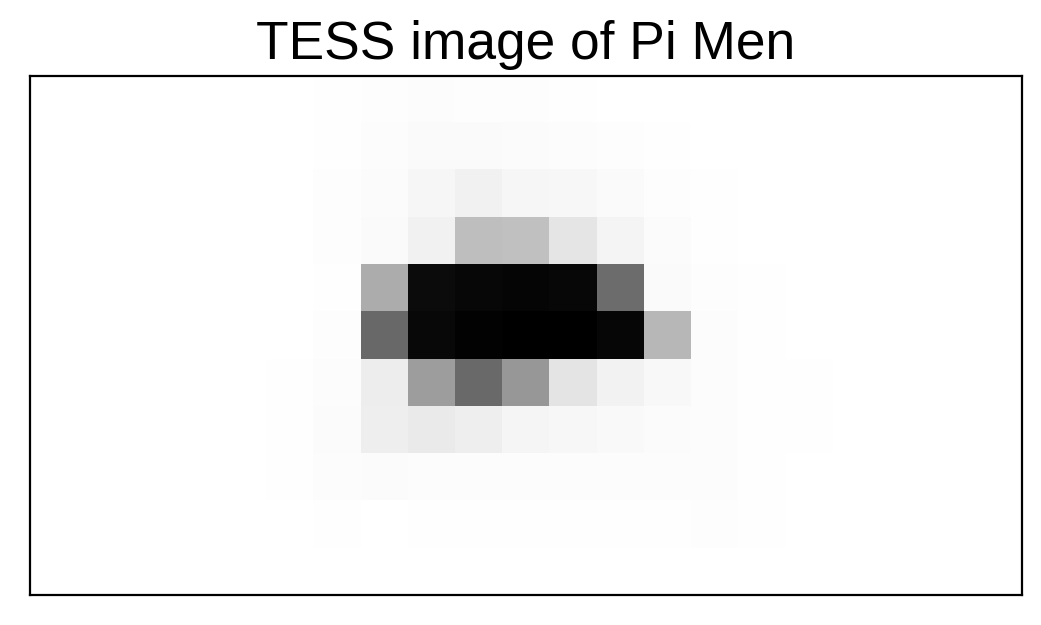
In this tutorial, we will reproduce the fits to the transiting planet in the Pi Mensae system discovered by Huang et al. (2018). The data processing and model are similar to the Case study: K2-24, putting it all together tutorial, but with a few extra bits like aperture selection and de-trending.
To start, we need to download the target pixel file:
import numpy as np
import lightkurve as lk
import matplotlib.pyplot as plt

tpf_file = lk.search_targetpixelfile("TIC 261136679", sector=1).download()
with tpf_file.hdu as hdu:
    tpf = hdu[1].data
    tpf_hdr = hdu[1].header

texp = tpf_hdr["FRAMETIM"] * tpf_hdr["NUM_FRM"]
texp /= 60.0 * 60.0 * 24.0
time = tpf["TIME"]
flux = tpf["FLUX"]
m = np.any(np.isfinite(flux), axis=(1, 2)) & (tpf["QUALITY"] == 0)
ref_time = 0.5 * (np.min(time[m]) + np.max(time[m]))
time = np.ascontiguousarray(time[m] - ref_time, dtype=np.float64)
flux = np.ascontiguousarray(flux[m], dtype=np.float64)

mean_img = np.median(flux, axis=0)
plt.imshow(mean_img.T, cmap="gray_r")
plt.title("TESS image of Pi Men")
plt.xticks([])
plt.yticks([]);
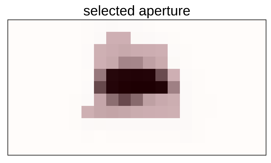
Next, we’ll select an aperture using a hacky method that tries to minimizes the windowed scatter in the lightcurve (something like the CDPP).
from scipy.signal import savgol_filter

# Sort the pixels by median brightness
order = np.argsort(mean_img.flatten())[::-1]

# A function to estimate the windowed scatter in a lightcurve
def estimate_scatter_with_mask(mask):
    f = np.sum(flux[:, mask], axis=-1)
    smooth = savgol_filter(f, 1001, polyorder=5)
    return 1e6 * np.sqrt(np.median((f / smooth - 1) ** 2))


# Loop over pixels ordered by brightness and add them one-by-one
# to the aperture
masks, scatters = [], []
for i in range(10, 100):
    msk = np.zeros_like(mean_img, dtype=bool)
    msk[np.unravel_index(order[:i], mean_img.shape)] = True
    scatter = estimate_scatter_with_mask(msk)
    masks.append(msk)
    scatters.append(scatter)

# Choose the aperture that minimizes the scatter
pix_mask = masks[np.argmin(scatters)]

# Plot the selected aperture
plt.imshow(mean_img.T, cmap="gray_r")
plt.imshow(pix_mask.T, cmap="Reds", alpha=0.3)
plt.title("selected aperture")
plt.xticks([])
plt.yticks([]);
This aperture produces the following light curve:
plt.figure(figsize=(10, 5))
sap_flux = np.sum(flux[:, pix_mask], axis=-1)
sap_flux = (sap_flux / np.median(sap_flux) - 1) * 1e3
plt.plot(time, sap_flux, "k")
plt.xlabel("time [days]")
plt.ylabel("relative flux [ppt]")
plt.title("raw light curve")
plt.xlim(time.min(), time.max());
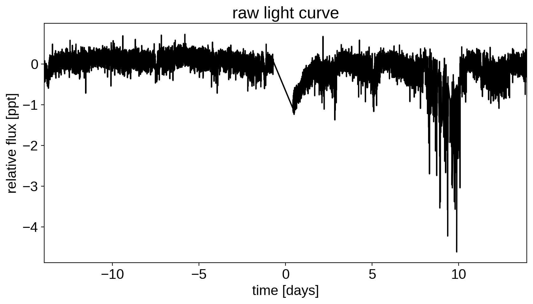
This doesn’t look terrible, but we’re still going to want to de-trend it a little bit. We’ll use “pixel-level deconvolution” (PLD) to de-trend following the method used by Everest. Specifically, we’ll use first order PLD plus the top few PCA components of the second order PLD basis.
# Build the first order PLD basis
X_pld = np.reshape(flux[:, pix_mask], (len(flux), -1))
X_pld = X_pld / np.sum(flux[:, pix_mask], axis=-1)[:, None]

# Build the second order PLD basis and run PCA to reduce the number of dimensions
X2_pld = np.reshape(X_pld[:, None, :] * X_pld[:, :, None], (len(flux), -1))
U, _, _ = np.linalg.svd(X2_pld, full_matrices=False)
X2_pld = U[:, : X_pld.shape[1]]

# Construct the design matrix and fit for the PLD model
X_pld = np.concatenate((np.ones((len(flux), 1)), X_pld, X2_pld), axis=-1)
XTX = np.dot(X_pld.T, X_pld)
w_pld = np.linalg.solve(XTX, np.dot(X_pld.T, sap_flux))
pld_flux = np.dot(X_pld, w_pld)

# Plot the de-trended light curve
plt.figure(figsize=(10, 5))
plt.plot(time, sap_flux - pld_flux, "k")
plt.xlabel("time [days]")
plt.ylabel("de-trended flux [ppt]")
plt.title("initial de-trended light curve")
plt.xlim(time.min(), time.max());
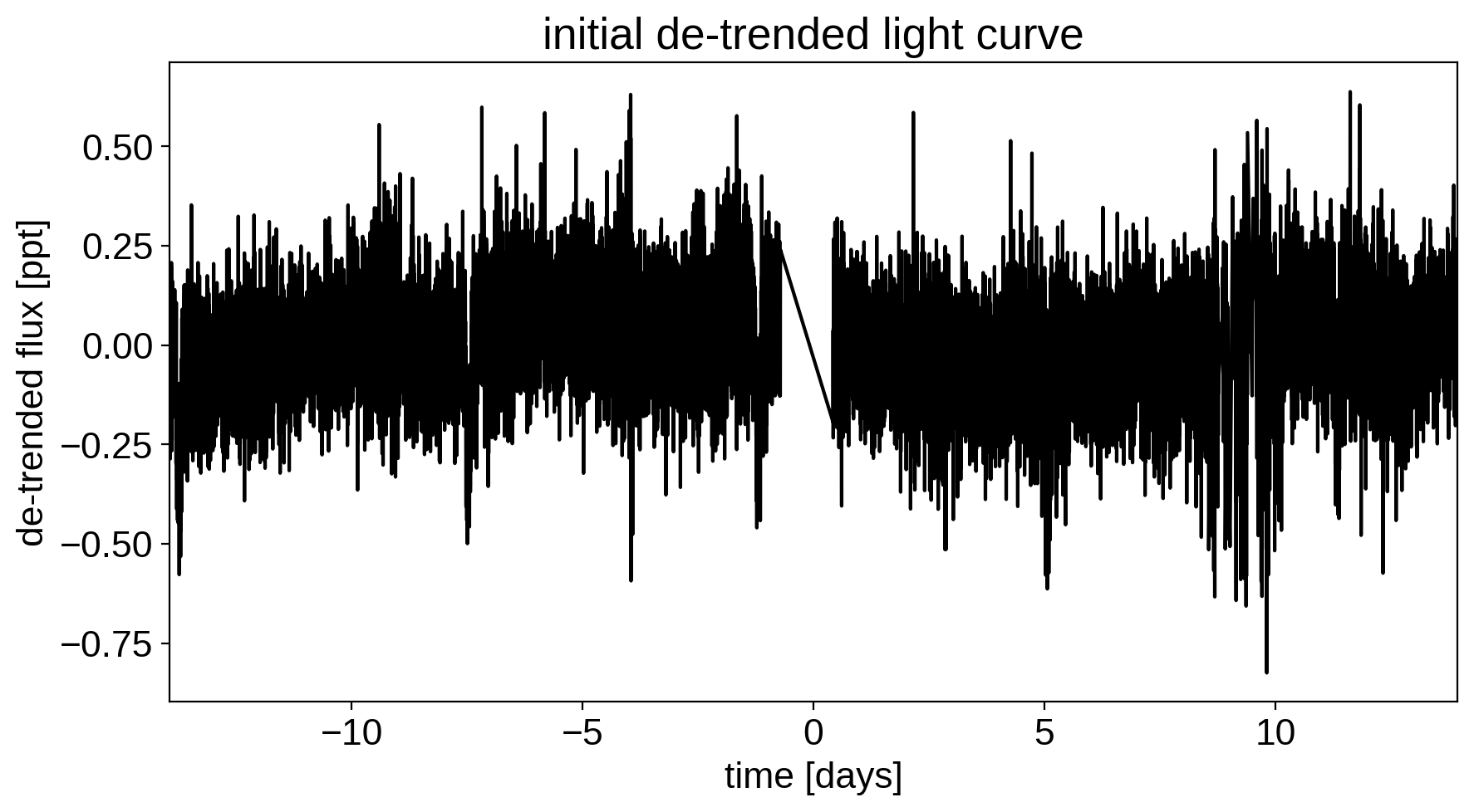
That looks better.
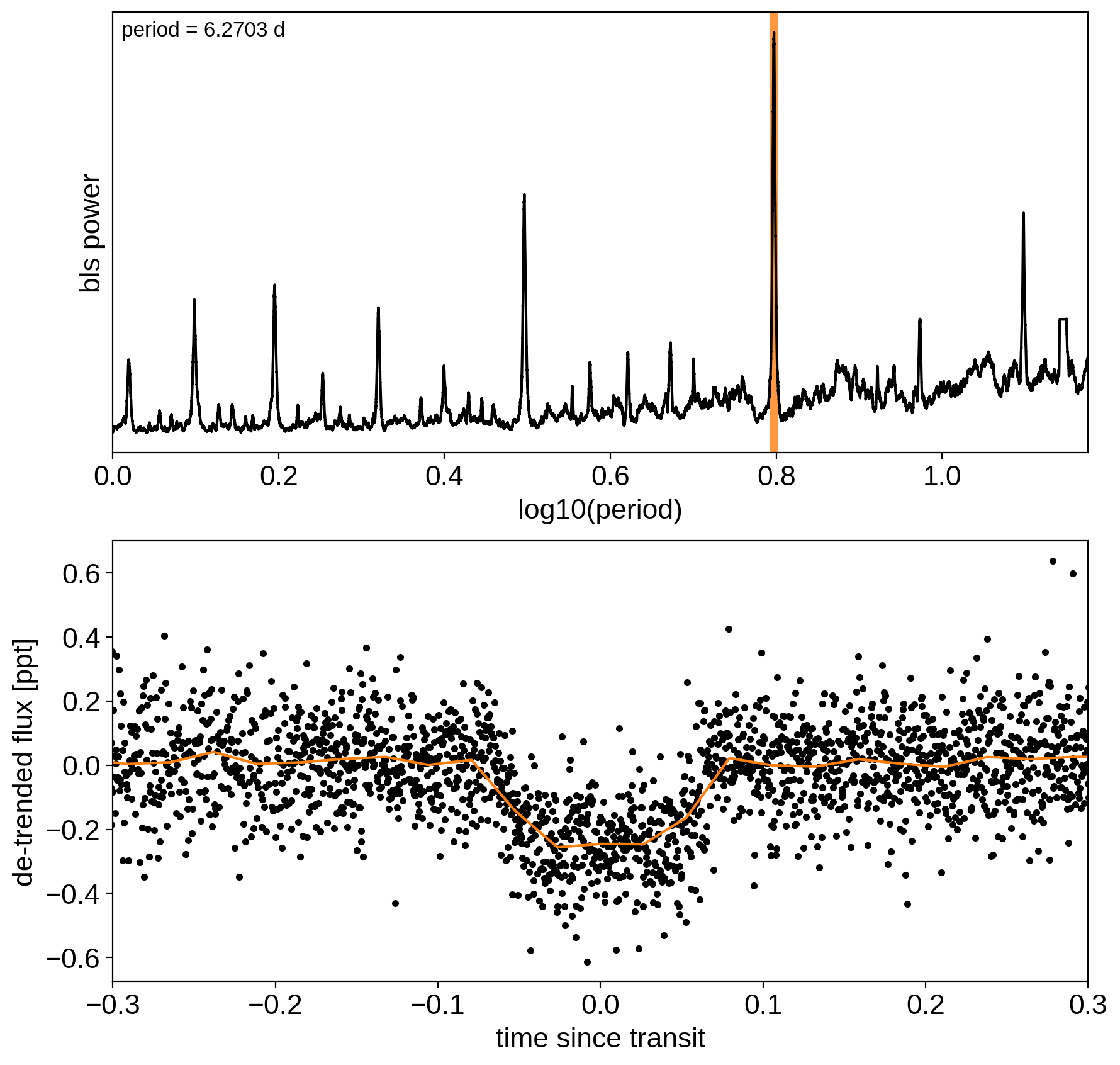
Now, let’s use the box least squares periodogram from AstroPy (Note: you’ll need AstroPy v3.1 or more recent to use this feature) to estimate the period, phase, and depth of the transit.
from astropy.timeseries import BoxLeastSquares

period_grid = np.exp(np.linspace(np.log(1), np.log(15), 50000))

bls = BoxLeastSquares(time, sap_flux - pld_flux)
bls_power = bls.power(period_grid, 0.1, oversample=20)

# Save the highest peak as the planet candidate
index = np.argmax(bls_power.power)
bls_period = bls_power.period[index]
bls_t0 = bls_power.transit_time[index]
bls_depth = bls_power.depth[index]
transit_mask = bls.transit_mask(time, bls_period, 0.2, bls_t0)

fig, axes = plt.subplots(2, 1, figsize=(10, 10))

# Plot the periodogram
ax = axes[0]
ax.axvline(np.log10(bls_period), color="C1", lw=5, alpha=0.8)
ax.plot(np.log10(bls_power.period), bls_power.power, "k")
ax.annotate(
    "period = {0:.4f} d".format(bls_period),
    (0, 1),
    xycoords="axes fraction",
    xytext=(5, -5),
    textcoords="offset points",
    va="top",
    ha="left",
    fontsize=12,
)
ax.set_ylabel("bls power")
ax.set_yticks([])
ax.set_xlim(np.log10(period_grid.min()), np.log10(period_grid.max()))
ax.set_xlabel("log10(period)")

# Plot the folded transit
ax = axes[1]
x_fold = (time - bls_t0 + 0.5 * bls_period) % bls_period - 0.5 * bls_period
m = np.abs(x_fold) < 0.4
ax.plot(x_fold[m], sap_flux[m] - pld_flux[m], ".k")

# Overplot the phase binned light curve
bins = np.linspace(-0.41, 0.41, 32)
denom, _ = np.histogram(x_fold, bins)
num, _ = np.histogram(x_fold, bins, weights=sap_flux - pld_flux)
denom[num == 0] = 1.0
ax.plot(0.5 * (bins[1:] + bins[:-1]), num / denom, color="C1")

ax.set_xlim(-0.3, 0.3)
ax.set_ylabel("de-trended flux [ppt]")
ax.set_xlabel("time since transit");
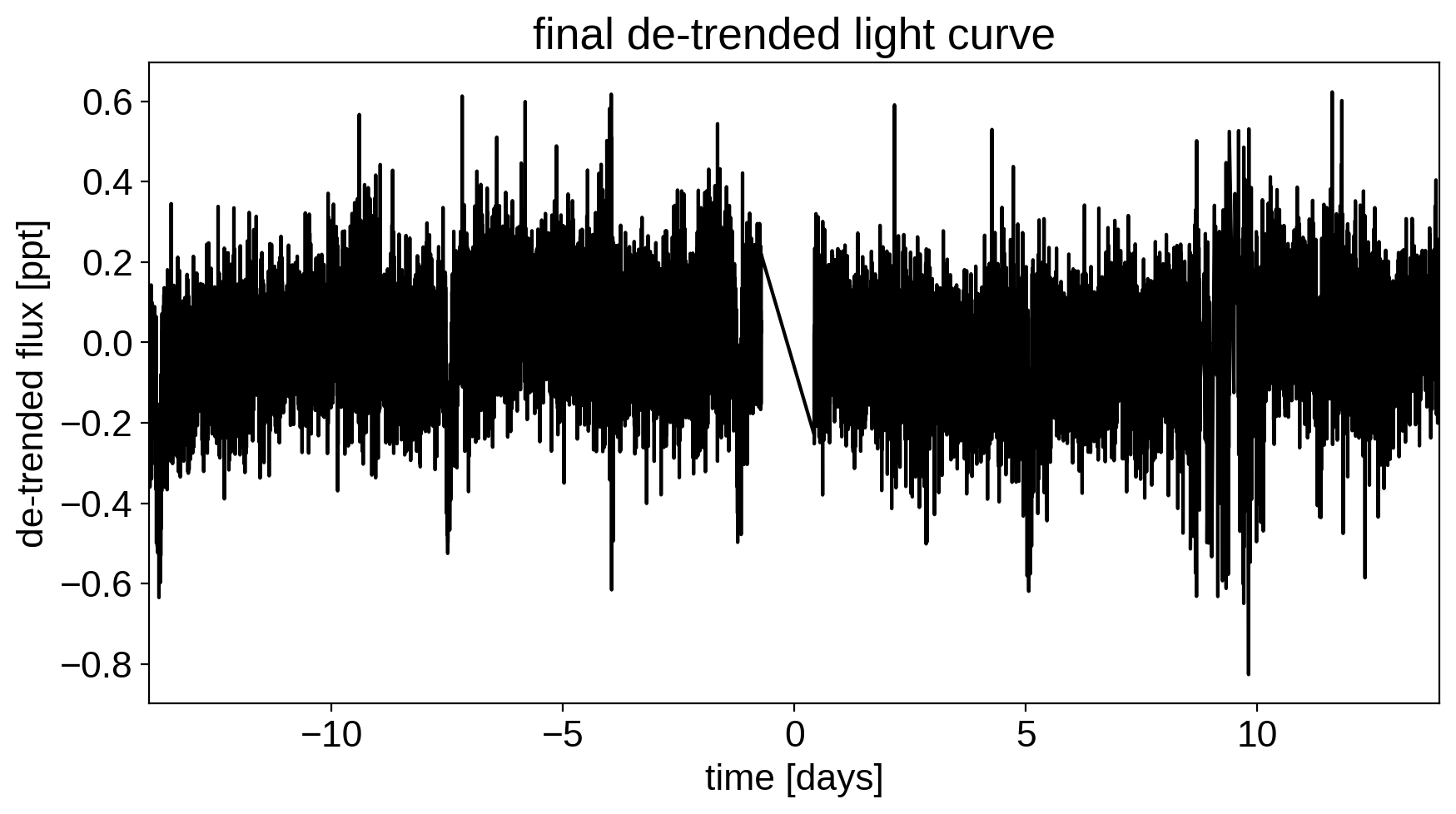
Now that we know where the transits are, it’s generally good practice to de-trend the data one more time with the transits masked so that the de-trending doesn’t overfit the transits. Let’s do that.
m = ~transit_mask
XTX = np.dot(X_pld[m].T, X_pld[m])
w_pld = np.linalg.solve(XTX, np.dot(X_pld[m].T, sap_flux[m]))
pld_flux = np.dot(X_pld, w_pld)

x = np.ascontiguousarray(time, dtype=np.float64)
y = np.ascontiguousarray(sap_flux - pld_flux, dtype=np.float64)

plt.figure(figsize=(10, 5))
plt.plot(time, y, "k")
plt.xlabel("time [days]")
plt.ylabel("de-trended flux [ppt]")
plt.title("final de-trended light curve")
plt.xlim(time.min(), time.max());
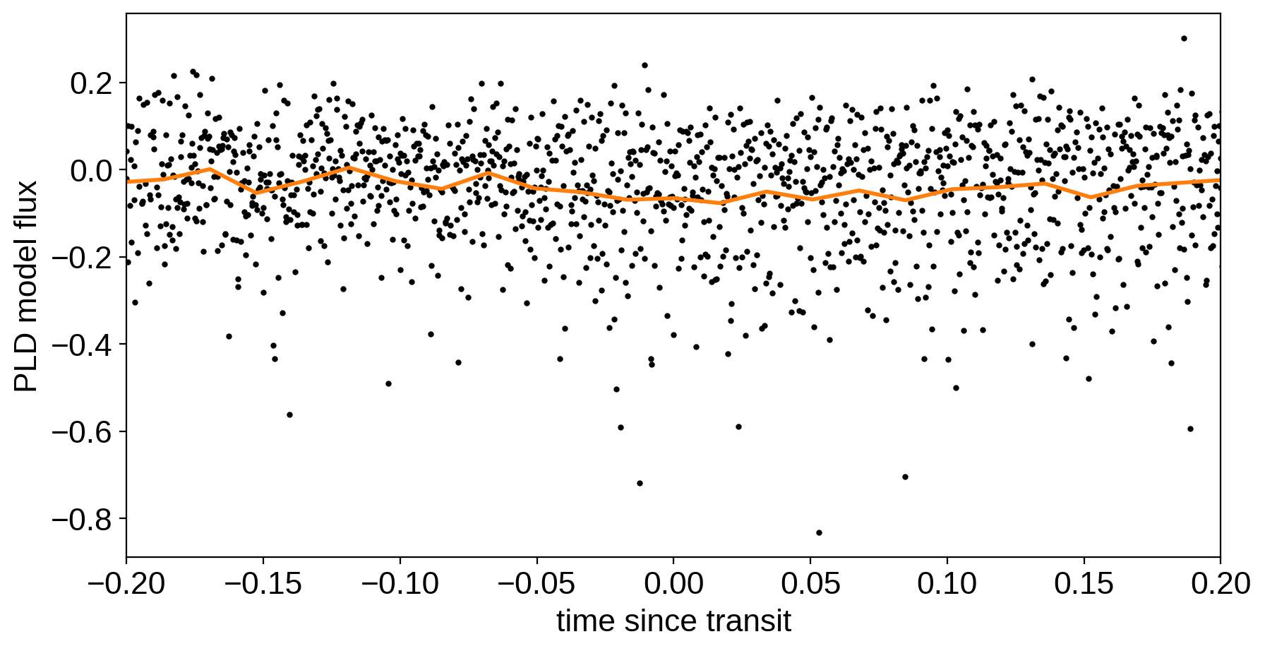
To confirm that we didn’t overfit the transit, we can look at the folded light curve for the PLD model near trasit. This shouldn’t have any residual transit signal, and that looks correct here:
plt.figure(figsize=(10, 5))

x_fold = (x - bls_t0 + 0.5 * bls_period) % bls_period - 0.5 * bls_period
m = np.abs(x_fold) < 0.3
plt.plot(x_fold[m], pld_flux[m], ".k", ms=4)

bins = np.linspace(-0.5, 0.5, 60)
denom, _ = np.histogram(x_fold, bins)
num, _ = np.histogram(x_fold, bins, weights=pld_flux)
denom[num == 0] = 1.0
plt.plot(0.5 * (bins[1:] + bins[:-1]), num / denom, color="C1", lw=2)
plt.xlim(-0.2, 0.2)
plt.xlabel("time since transit")
plt.ylabel("PLD model flux");
The transit model, initialization, and sampling are all nearly the same as the one in Case study: K2-24, putting it all together.
import exoplanet as xo
import pymc3 as pm
import theano.tensor as tt


def build_model(mask=None, start=None):
    if mask is None:
        mask = np.ones(len(x), dtype=bool)
    with pm.Model() as model:

        # Parameters for the stellar properties
        mean = pm.Normal("mean", mu=0.0, sd=10.0)
        u_star = xo.distributions.QuadLimbDark("u_star")

        # Stellar parameters from Huang et al (2018)
        M_star_huang = 1.094, 0.039
        R_star_huang = 1.10, 0.023
        BoundedNormal = pm.Bound(pm.Normal, lower=0, upper=3)
        m_star = BoundedNormal("m_star", mu=M_star_huang[0], sd=M_star_huang[1])
        r_star = BoundedNormal("r_star", mu=R_star_huang[0], sd=R_star_huang[1])

        # Orbital parameters for the planets
        logP = pm.Normal("logP", mu=np.log(bls_period), sd=1)
        t0 = pm.Normal("t0", mu=bls_t0, sd=1)
        logr = pm.Normal(
            "logr",
            sd=1.0,
            mu=0.5 * np.log(1e-3 * np.array(bls_depth)) + np.log(R_star_huang[0]),
        )
        r_pl = pm.Deterministic("r_pl", tt.exp(logr))
        ror = pm.Deterministic("ror", r_pl / r_star)
        b = xo.distributions.ImpactParameter("b", ror=ror)

        ecs = xo.UnitDisk("ecs", testval=np.array([0.01, 0.0]))
        ecc = pm.Deterministic("ecc", tt.sum(ecs ** 2))
        omega = pm.Deterministic("omega", tt.arctan2(ecs[1], ecs[0]))
        xo.eccentricity.kipping13("ecc_prior", observed=ecc)

        # Transit jitter & GP parameters
        logs2 = pm.Normal("logs2", mu=np.log(np.var(y[mask])), sd=10)
        logw0 = pm.Normal("logw0", mu=0, sd=10)
        logSw4 = pm.Normal("logSw4", mu=np.log(np.var(y[mask])), sd=10)

        # Tracking planet parameters
        period = pm.Deterministic("period", tt.exp(logP))

        # Orbit model
        orbit = xo.orbits.KeplerianOrbit(
            r_star=r_star,
            m_star=m_star,
            period=period,
            t0=t0,
            b=b,
            ecc=ecc,
            omega=omega,
        )

        def mean_model(t):
            # Compute the model light curve using starry
            light_curves = pm.Deterministic(
                "light_curves",
                xo.LimbDarkLightCurve(u_star).get_light_curve(
                    orbit=orbit, r=r_pl, t=t, texp=texp
                )
                * 1e3,
            )
            return tt.sum(light_curves, axis=-1) + mean

        # GP model for the light curve
        kernel = xo.gp.terms.SHOTerm(log_Sw4=logSw4, log_w0=logw0, Q=1 / np.sqrt(2))
        gp = xo.gp.GP(
            kernel, x[mask], tt.exp(logs2) + tt.zeros(mask.sum()), mean=mean_model
        )
        gp.marginal("gp", observed=y[mask])
        pm.Deterministic("gp_pred", gp.predict())

        # Fit for the maximum a posteriori parameters, I've found that I can get
        # a better solution by trying different combinations of parameters in turn
        if start is None:
            start = model.test_point
        map_soln = xo.optimize(start=start, vars=[logs2, logSw4, logw0])
        map_soln = xo.optimize(start=map_soln, vars=[logr])
        map_soln = xo.optimize(start=map_soln, vars=[b])
        map_soln = xo.optimize(start=map_soln, vars=[logP, t0])
        map_soln = xo.optimize(start=map_soln, vars=[u_star])
        map_soln = xo.optimize(start=map_soln, vars=[logr])
        map_soln = xo.optimize(start=map_soln, vars=[b])
        map_soln = xo.optimize(start=map_soln, vars=[ecc, omega])
        map_soln = xo.optimize(start=map_soln, vars=[mean])
        map_soln = xo.optimize(start=map_soln, vars=[logs2, logSw4, logw0])
        map_soln = xo.optimize(start=map_soln)

    return model, map_soln


model0, map_soln0 = build_model()
optimizing logp for variables: [logw0, logSw4, logs2]
34it [00:08,  3.79it/s, logp=1.264106e+04]
message: Desired error not necessarily achieved due to precision loss.
logp: 12405.224536471058 -> 12641.06206967105
optimizing logp for variables: [logr]
264it [00:03, 71.24it/s, logp=1.267895e+04]
message: Desired error not necessarily achieved due to precision loss.
logp: 12641.062069671045 -> 12678.952985094724
optimizing logp for variables: [b, logr, r_star]
84it [00:02, 32.21it/s, logp=1.295053e+04]
message: Desired error not necessarily achieved due to precision loss.
logp: 12678.952985094724 -> 12950.529848063012
optimizing logp for variables: [t0, logP]
22it [00:02,  9.36it/s, logp=1.296485e+04]
message: Optimization terminated successfully.
logp: 12950.529848063008 -> 12964.849107164231
optimizing logp for variables: [u_star]
11it [00:01,  5.70it/s, logp=1.296772e+04]
message: Optimization terminated successfully.
logp: 12964.849107164227 -> 12967.719850225458
optimizing logp for variables: [logr]
9it [00:01,  5.28it/s, logp=1.296789e+04]
message: Optimization terminated successfully.
logp: 12967.719850225465 -> 12967.894818446483
optimizing logp for variables: [b, logr, r_star]
117it [00:02, 39.37it/s, logp=1.296803e+04]
message: Desired error not necessarily achieved due to precision loss.
logp: 12967.894818446483 -> 12968.027872730941
optimizing logp for variables: [ecs]
15it [00:01,  8.47it/s, logp=1.296860e+04]
message: Optimization terminated successfully.
logp: 12968.027872730941 -> 12968.59732823194
optimizing logp for variables: [mean]
5it [00:01,  3.50it/s, logp=1.296863e+04]
message: Optimization terminated successfully.
logp: 12968.597328231934 -> 12968.625555627523
optimizing logp for variables: [logw0, logSw4, logs2]
91it [00:02, 39.44it/s, logp=1.297926e+04]
message: Desired error not necessarily achieved due to precision loss.
logp: 12968.625555627523 -> 12979.264919901398
optimizing logp for variables: [logSw4, logw0, logs2, ecc_prior_beta, ecc_prior_alpha, ecs, b, logr, t0, logP, r_star, m_star, u_star, mean]
132it [00:02, 49.23it/s, logp=1.303527e+04]
message: Desired error not necessarily achieved due to precision loss.
logp: 12979.264919901387 -> 13035.272557029253
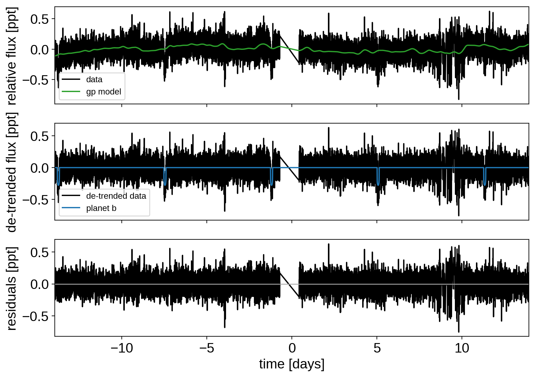
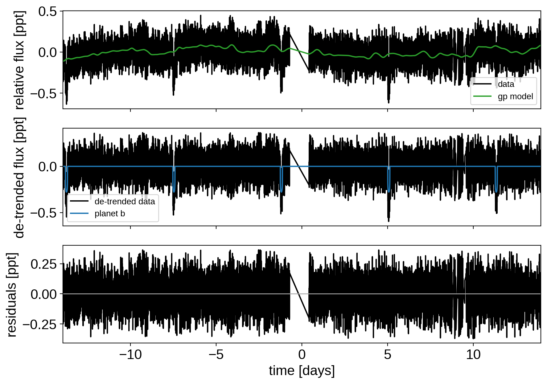
Here’s how we plot the initial light curve model:
def plot_light_curve(soln, mask=None):
    if mask is None:
        mask = np.ones(len(x), dtype=bool)

    fig, axes = plt.subplots(3, 1, figsize=(10, 7), sharex=True)

    ax = axes[0]
    ax.plot(x[mask], y[mask], "k", label="data")
    gp_mod = soln["gp_pred"] + soln["mean"]
    ax.plot(x[mask], gp_mod, color="C2", label="gp model")
    ax.legend(fontsize=10)
    ax.set_ylabel("relative flux [ppt]")

    ax = axes[1]
    ax.plot(x[mask], y[mask] - gp_mod, "k", label="de-trended data")
    for i, l in enumerate("b"):
        mod = soln["light_curves"][:, i]
        ax.plot(x[mask], mod, label="planet {0}".format(l))
    ax.legend(fontsize=10, loc=3)
    ax.set_ylabel("de-trended flux [ppt]")

    ax = axes[2]
    mod = gp_mod + np.sum(soln["light_curves"], axis=-1)
    ax.plot(x[mask], y[mask] - mod, "k")
    ax.axhline(0, color="#aaaaaa", lw=1)
    ax.set_ylabel("residuals [ppt]")
    ax.set_xlim(x[mask].min(), x[mask].max())
    ax.set_xlabel("time [days]")

    return fig


plot_light_curve(map_soln0);
As in the Case study: K2-24, putting it all together tutorial, we can do some sigma clipping to remove significant outliers.
mod = (
    map_soln0["gp_pred"]
    + map_soln0["mean"]
    + np.sum(map_soln0["light_curves"], axis=-1)
)
resid = y - mod
rms = np.sqrt(np.median(resid ** 2))
mask = np.abs(resid) < 5 * rms

plt.figure(figsize=(10, 5))
plt.plot(x, resid, "k", label="data")
plt.plot(x[~mask], resid[~mask], "xr", label="outliers")
plt.axhline(0, color="#aaaaaa", lw=1)
plt.ylabel("residuals [ppt]")
plt.xlabel("time [days]")
plt.legend(fontsize=12, loc=3)
plt.xlim(x.min(), x.max());
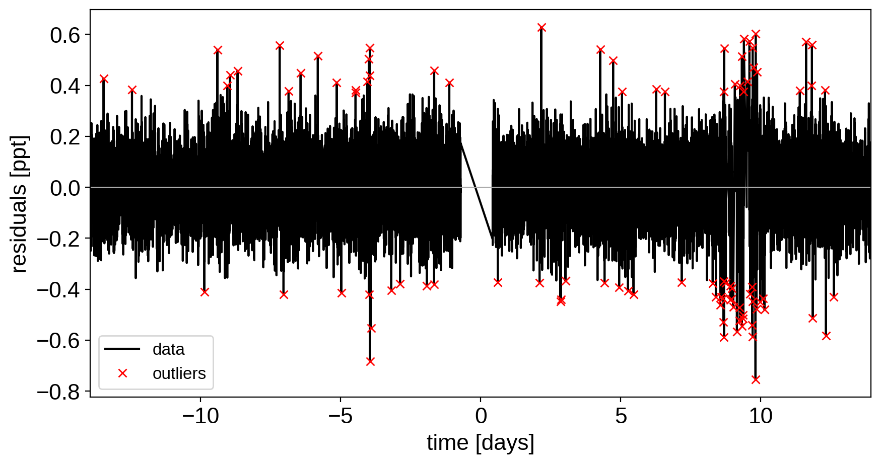
And then we re-build the model using the data without outliers.
model, map_soln = build_model(mask, map_soln0)
plot_light_curve(map_soln, mask);
optimizing logp for variables: [logw0, logSw4, logs2]
15it [00:01, 10.80it/s, logp=1.372057e+04]
message: Optimization terminated successfully.
logp: 13689.624267247154 -> 13720.569965671924
optimizing logp for variables: [logr]
8it [00:01,  5.81it/s, logp=1.372059e+04]
message: Optimization terminated successfully.
logp: 13720.569965671928 -> 13720.590200785264
optimizing logp for variables: [b, logr, r_star]
48it [00:01, 29.65it/s, logp=1.372059e+04]
message: Desired error not necessarily achieved due to precision loss.
logp: 13720.590200785264 -> 13720.590906642601
optimizing logp for variables: [t0, logP]
93it [00:02, 37.69it/s, logp=1.372060e+04]
message: Desired error not necessarily achieved due to precision loss.
logp: 13720.590906642605 -> 13720.59859489801
optimizing logp for variables: [u_star]
8it [00:01,  6.43it/s, logp=1.372062e+04]
message: Optimization terminated successfully.
logp: 13720.59859489801 -> 13720.624962714914
optimizing logp for variables: [logr]
8it [00:01,  5.90it/s, logp=1.372063e+04]
message: Optimization terminated successfully.
logp: 13720.624962714912 -> 13720.627429857885
optimizing logp for variables: [b, logr, r_star]
13it [00:01,  9.63it/s, logp=1.372064e+04]
message: Optimization terminated successfully.
logp: 13720.627429857885 -> 13720.63764856563
optimizing logp for variables: [ecs]
12it [00:01,  9.69it/s, logp=1.372064e+04]
message: Optimization terminated successfully.
logp: 13720.637648565627 -> 13720.637655387956
optimizing logp for variables: [mean]
5it [00:01,  4.13it/s, logp=1.372064e+04]
message: Optimization terminated successfully.
logp: 13720.637655387955 -> 13720.64083013365
optimizing logp for variables: [logw0, logSw4, logs2]
9it [00:01,  5.33it/s, logp=1.372064e+04]
message: Optimization terminated successfully.
logp: 13720.64083013365 -> 13720.640833096417
optimizing logp for variables: [logSw4, logw0, logs2, ecc_prior_beta, ecc_prior_alpha, ecs, b, logr, t0, logP, r_star, m_star, u_star, mean]
124it [00:02, 49.43it/s, logp=1.372065e+04]
message: Desired error not necessarily achieved due to precision loss.
logp: 13720.64083309642 -> 13720.647587016902
Now that we have the model, we can sample:
np.random.seed(261136679)
with model:
    trace = xo.sample(
        tune=3500, draws=3000, start=map_soln, chains=4, target_accept=0.95
    )
Multiprocess sampling (4 chains in 4 jobs)
NUTS: [logSw4, logw0, logs2, ecc_prior_beta, ecc_prior_alpha, ecs, b, logr, t0, logP, r_star, m_star, u_star, mean]
Sampling 4 chains, 0 divergences: 100%|██████████| 26000/26000 [2:36:08<00:00,  2.78draws/s]
The number of effective samples is smaller than 25% for some parameters.
pm.summary(
    trace,
    var_names=[
        "logw0",
        "logSw4",
        "logs2",
        "omega",
        "ecc",
        "r_pl",
        "b",
        "t0",
        "logP",
        "r_star",
        "m_star",
        "u_star",
        "mean",
    ],
)
| mean | sd | hpd_3% | hpd_97% | mcse_mean | mcse_sd | ess_mean | ess_sd | ess_bulk | ess_tail | r_hat | |
|---|---|---|---|---|---|---|---|---|---|---|---|
| logw0 | 1.177 | 0.136 | 0.918 | 1.430 | 0.001 | 0.001 | 8295.0 | 8295.0 | 8604.0 | 7666.0 | 1.0 |
| logSw4 | -2.105 | 0.318 | -2.684 | -1.487 | 0.003 | 0.002 | 9509.0 | 9509.0 | 9488.0 | 8245.0 | 1.0 |
| logs2 | -4.383 | 0.011 | -4.404 | -4.363 | 0.000 | 0.000 | 12555.0 | 12555.0 | 12561.0 | 8701.0 | 1.0 |
| omega | 0.664 | 1.733 | -2.763 | 3.141 | 0.027 | 0.019 | 4104.0 | 4104.0 | 5404.0 | 8554.0 | 1.0 |
| ecc | 0.227 | 0.150 | 0.000 | 0.498 | 0.003 | 0.003 | 2041.0 | 1121.0 | 3111.0 | 1929.0 | 1.0 |
| r_pl | 0.017 | 0.001 | 0.016 | 0.018 | 0.000 | 0.000 | 3279.0 | 3173.0 | 3969.0 | 2999.0 | 1.0 |
| b | 0.393 | 0.219 | 0.000 | 0.720 | 0.004 | 0.003 | 2742.0 | 2465.0 | 2451.0 | 2526.0 | 1.0 |
| t0 | -13.733 | 0.001 | -13.735 | -13.730 | 0.000 | 0.000 | 1085.0 | 1085.0 | 4211.0 | 2064.0 | 1.0 |
| logP | 1.835 | 0.000 | 1.835 | 1.836 | 0.000 | 0.000 | 7839.0 | 7839.0 | 8185.0 | 8893.0 | 1.0 |
| r_star | 1.098 | 0.023 | 1.055 | 1.141 | 0.000 | 0.000 | 11224.0 | 11224.0 | 11225.0 | 9070.0 | 1.0 |
| m_star | 1.095 | 0.039 | 1.024 | 1.170 | 0.000 | 0.000 | 12738.0 | 12738.0 | 12726.0 | 8281.0 | 1.0 |
| u_star[0] | 0.203 | 0.170 | 0.000 | 0.515 | 0.002 | 0.002 | 6352.0 | 4685.0 | 6755.0 | 5955.0 | 1.0 |
| u_star[1] | 0.454 | 0.275 | -0.080 | 0.919 | 0.004 | 0.003 | 5446.0 | 5446.0 | 5280.0 | 6082.0 | 1.0 |
| mean | -0.001 | 0.009 | -0.018 | 0.016 | 0.000 | 0.000 | 9308.0 | 5329.0 | 9440.0 | 7443.0 | 1.0 |
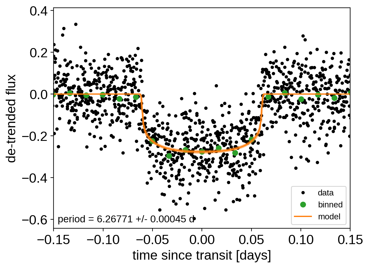
After sampling, we can make the usual plots. First, let’s look at the folded light curve plot:
# Compute the GP prediction
gp_mod = np.median(trace["gp_pred"] + trace["mean"][:, None], axis=0)

# Get the posterior median orbital parameters
p = np.median(trace["period"])
t0 = np.median(trace["t0"])

# Plot the folded data
x_fold = (x[mask] - t0 + 0.5 * p) % p - 0.5 * p
plt.plot(x_fold, y[mask] - gp_mod, ".k", label="data", zorder=-1000)

# Overplot the phase binned light curve
bins = np.linspace(-0.41, 0.41, 50)
denom, _ = np.histogram(x_fold, bins)
num, _ = np.histogram(x_fold, bins, weights=y[mask])
denom[num == 0] = 1.0
plt.plot(0.5 * (bins[1:] + bins[:-1]), num / denom, "o", color="C2", label="binned")

# Plot the folded model
inds = np.argsort(x_fold)
inds = inds[np.abs(x_fold)[inds] < 0.3]
pred = trace["light_curves"][:, inds, 0]
pred = np.percentile(pred, [16, 50, 84], axis=0)
plt.plot(x_fold[inds], pred[1], color="C1", label="model")
art = plt.fill_between(
    x_fold[inds], pred[0], pred[2], color="C1", alpha=0.5, zorder=1000
)
art.set_edgecolor("none")

# Annotate the plot with the planet's period
txt = "period = {0:.5f} +/- {1:.5f} d".format(
    np.mean(trace["period"]), np.std(trace["period"])
)
plt.annotate(
    txt,
    (0, 0),
    xycoords="axes fraction",
    xytext=(5, 5),
    textcoords="offset points",
    ha="left",
    va="bottom",
    fontsize=12,
)

plt.legend(fontsize=10, loc=4)
plt.xlim(-0.5 * p, 0.5 * p)
plt.xlabel("time since transit [days]")
plt.ylabel("de-trended flux")
plt.xlim(-0.15, 0.15);
And a corner plot of some of the key parameters:
import corner
import astropy.units as u

varnames = ["period", "b", "ecc", "r_pl"]
samples = pm.trace_to_dataframe(trace, varnames=varnames)

# Convert the radius to Earth radii
samples["r_pl"] = (np.array(samples["r_pl"]) * u.R_sun).to(u.R_earth).value

corner.corner(
    samples[["period", "r_pl", "b", "ecc"]],
    labels=["period [days]", "radius [Earth radii]", "impact param", "eccentricity"],
);
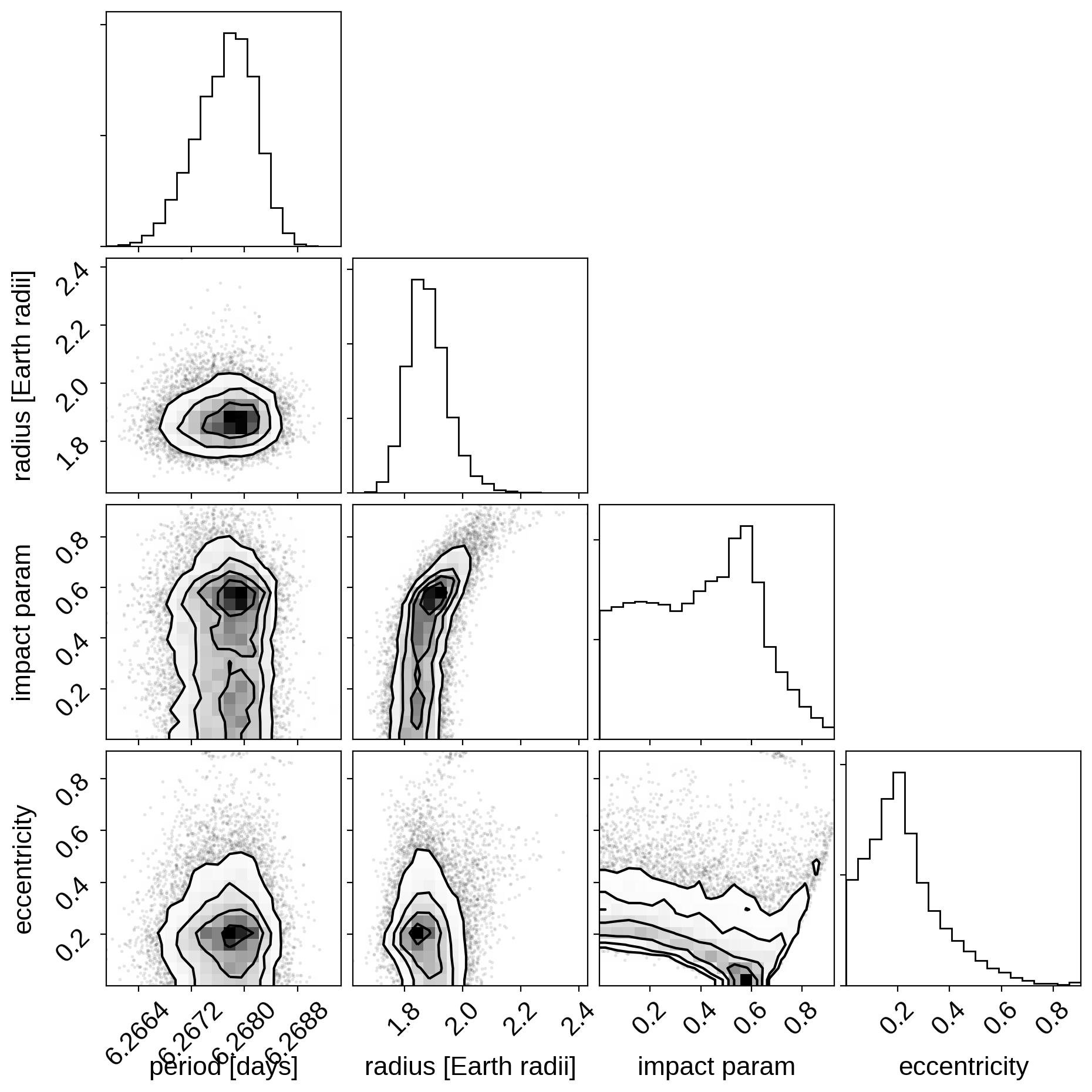
These all seem consistent with the previously published values and an earlier inconsistency between this radius measurement and the literature has been resolved by fixing a bug in exoplanet.
As described in the Citing exoplanet & its dependencies tutorial, we can use
exoplanet.citations.get_citations_for_model() to construct an
acknowledgement and BibTeX listing that includes the relevant citations
for this model.
with model:
    txt, bib = xo.citations.get_citations_for_model()
print(txt)
This research made use of textsf{exoplanet} citep{exoplanet} and its
dependencies citep{exoplanet:agol19, exoplanet:astropy13, exoplanet:astropy18,
exoplanet:exoplanet, exoplanet:foremanmackey17, exoplanet:foremanmackey18,
exoplanet:kipping13, exoplanet:kipping13b, exoplanet:luger18, exoplanet:pymc3,
exoplanet:theano}.
print("\n".join(bib.splitlines()[:10]) + "\n...")
@misc{exoplanet:exoplanet,
  author = {Daniel Foreman-Mackey and Rodrigo Luger and Ian Czekala and
            Eric Agol and Adrian Price-Whelan and Tom Barclay},
   title = {exoplanet-dev/exoplanet v0.3.2},
   month = may,
    year = 2020,
     doi = {10.5281/zenodo.1998447},
     url = {https://doi.org/10.5281/zenodo.1998447}
}
...