Note
This tutorial was generated from an IPython notebook that can be downloaded here.
In the RVs with multiple instruments case study, we discussed fitting the radial velocity curve for a planetary system observed using multiple instruments. You might also want to fit data from multiple instruments when fitting the light curve of a transiting planet and that’s what we work through in this example. This is a somewhat more complicated example than the radial velocity case because some of the physical properties of the system can vary as as function of the instrument. Specifically, the transit depth (or the effective raduis of the planet) will be a function of the filter or effective wavelength of the observations. This is the idea behind transit spectroscopy and the method used in this case study could (and should!) be extended to that use case. In this case, we’ll combine the light curves from the Kepler and TESS missions for the planet host HAT-P-11.
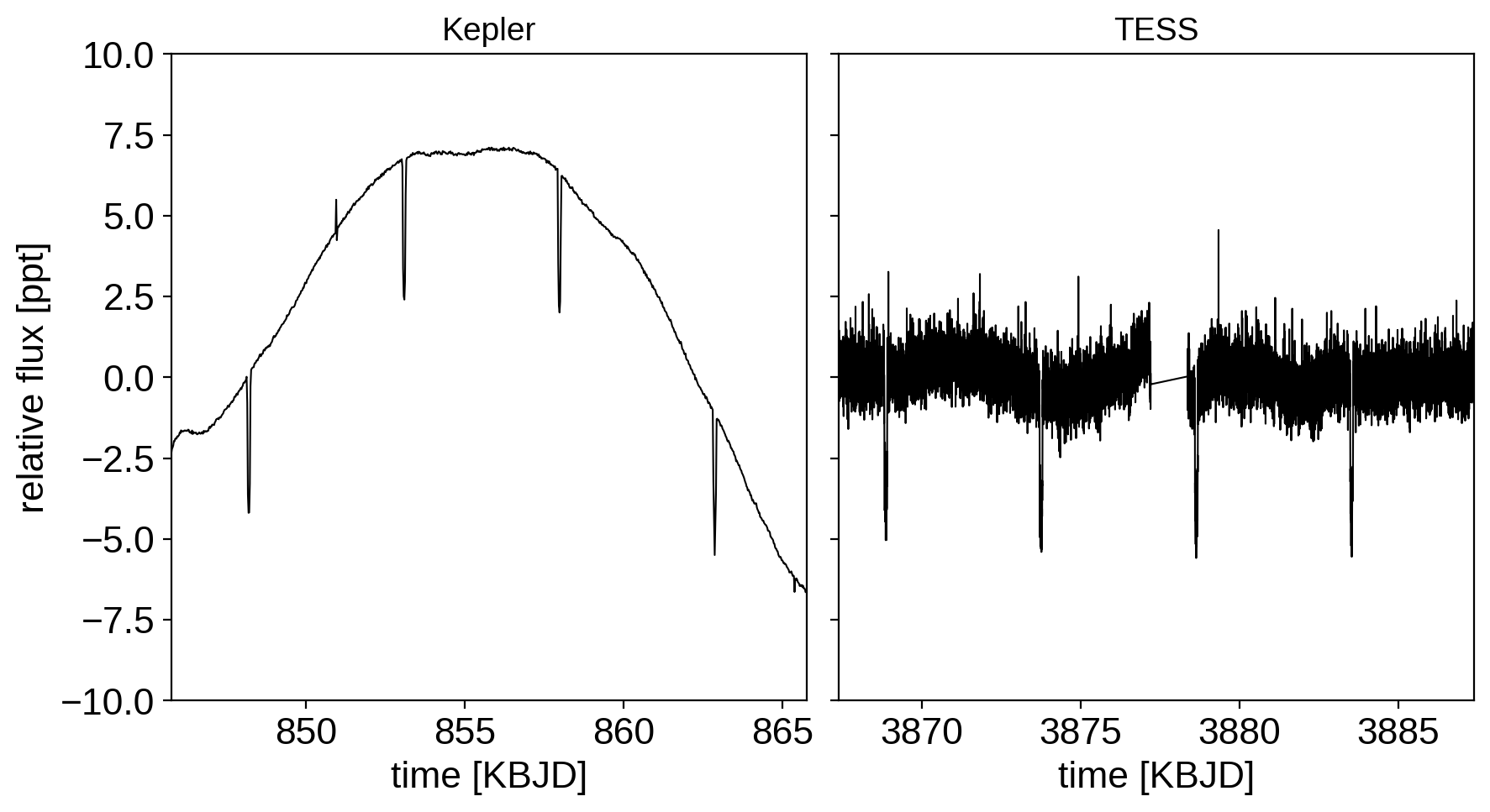
Before getting into the details of this case study, let’s spend a minute talking about a topic that comes up a lot when discussing combining observations from different instruments or techniques. To many people, it seems intuitive that one should (and perhaps must) “weight” how much each dataset contributes to the likelihood based on how much they “trust” those data. For example, you might be worried that a dataset with more datapoints will have a larger effect on the the results than you would like. While this might seem intuitive, it’s wrong: the only way to combine datasets is to multiply their likelihood functions. Instead, it is useful to understand what you actually mean when you say that you don’t “trust” a dataset as much as another. What you’re really saying is that you don’t believe the observation model that you wrote down. For example, you might think that the quoted error bars are underestimated or there might be correlated noise that an uncorrelated normal observation model can’t capture. The benefit of thinking about it this way is that it suggests a solution to the problem: incorporate a more flexible observation model that can capture these issues. In this case study, the 4 years of (long-cadence) Kepler observations only include about two times as many data points as one month of TESS observations. But, as you can see in the figure below, these two datasets have different noise properties (both in terms of photon noise and correlated noise) so we will fit using a different flexible Gaussian process noise model for each data set that will take these different properties into account.
import numpy as np
import lightkurve as lk
from collections import OrderedDict

kepler_lcfs = lk.search_lightcurvefile("HAT-P-11", mission="Kepler").download_all()
kepler_lc = kepler_lcfs.PDCSAP_FLUX.stitch().remove_nans()
kepler_t = np.ascontiguousarray(kepler_lc.time, dtype=np.float64)
kepler_y = np.ascontiguousarray(1e3 * (kepler_lc.flux - 1), dtype=np.float64)
kepler_yerr = np.ascontiguousarray(1e3 * kepler_lc.flux_err, dtype=np.float64)

hdr = kepler_lcfs[0].hdu[1].header
kepler_texp = hdr["FRAMETIM"] * hdr["NUM_FRM"]
kepler_texp /= 60.0 * 60.0 * 24.0

tess_lcfs = lk.search_lightcurvefile("HAT-P-11", mission="TESS").download_all()
tess_lc = tess_lcfs.PDCSAP_FLUX.stitch().remove_nans()
tess_t = np.ascontiguousarray(tess_lc.time + 2457000 - 2454833, dtype=np.float64)
tess_y = np.ascontiguousarray(1e3 * (tess_lc.flux - 1), dtype=np.float64)
tess_yerr = np.ascontiguousarray(1e3 * tess_lc.flux_err, dtype=np.float64)

hdr = tess_lcfs[0].hdu[1].header
tess_texp = hdr["FRAMETIM"] * hdr["NUM_FRM"]
tess_texp /= 60.0 * 60.0 * 24.0

datasets = OrderedDict(
    [
        ("Kepler", [kepler_t, kepler_y, kepler_yerr, kepler_texp]),
        ("TESS", [tess_t, tess_y, tess_yerr, tess_texp]),
    ]
)

fig, axes = plt.subplots(1, len(datasets), sharey=True, figsize=(10, 5))

for i, (name, (t, y, _, _)) in enumerate(datasets.items()):
    ax = axes[i]
    ax.plot(t, y, "k", lw=0.75, label=name)
    ax.set_xlabel("time [KBJD]")
    ax.set_title(name, fontsize=14)

    x_mid = 0.5 * (t.min() + t.max())
    ax.set_xlim(x_mid - 10, x_mid + 10)
axes[0].set_ylim(-10, 10)
fig.subplots_adjust(wspace=0.05)
_ = axes[0].set_ylabel("relative flux [ppt]")
This model is mostly the same as the one used in Quick fits for TESS light curves,
but we’re allowing for different noise variances (both the white noise
component and the GP amplitude), effective planet radii, and
limb-darkening coeeficients for each dataset. For the purposes of
demonstration, we’re sharing the length scale of the GP between the two
datasets, but this could just have well been a different parameter for
each dataset without changing the results. The final change that we’re
using is to use the approximate transit depth approx_depth (the
depth of the transit at minimum assuming the limb-darkening profile is
constant under the disk of the planet) as a parameter instead of the
radius ratio. This does not have a large effect on the performance or
the results, but it can sometimes be a useful parameterization when
dealing with high signal-to-noise transits because it reduces the
covariance between the radius parameter and the limb darkening
coefficients. As usual, we run a few iterations of sigma clipping and
then find the maximum a posteriori parameters to check to make sure that
everything is working:
import pymc3 as pm
import exoplanet as xo
import theano.tensor as tt
from functools import partial

# Period and reference transit time from the literature for initialization
lit_period = 4.887803076
lit_t0 = 124.8130808

# Find a reference transit time near the middle of the observations to avoid
# strong covariances between period and t0
x_min = min(np.min(x) for x, _, _, _ in datasets.values())
x_max = max(np.max(x) for x, _, _, _ in datasets.values())
x_mid = 0.5 * (x_min + x_max)
t0_ref = lit_t0 + lit_period * np.round((x_mid - lit_t0) / lit_period)

# Do several rounds of sigma clipping
for i in range(10):
    with pm.Model() as model:

        # Shared orbital parameters
        period = pm.Lognormal("period", mu=np.log(lit_period), sigma=1.0)
        t0 = pm.Normal("t0", mu=t0_ref, sigma=1.0)
        dur = pm.Lognormal("dur", mu=np.log(0.1), sigma=10.0)
        b = xo.UnitUniform("b")
        ld_arg = 1 - tt.sqrt(1 - b ** 2)
        orbit = xo.orbits.KeplerianOrbit(period=period, duration=dur, t0=t0, b=b)

        # We'll also say that the timescale of the GP will be shared
        ell = pm.InverseGamma(
            "ell", testval=2.0, **xo.estimate_inverse_gamma_parameters(1.0, 5.0)
        )

        # Loop over the instruments
        parameters = dict()
        lc_models = dict()
        gp_preds = dict()
        gp_preds_with_mean = dict()
        for n, (name, (x, y, yerr, texp)) in enumerate(datasets.items()):

            # We define the per-instrument parameters in a submodel so that we
            # don't have to prefix the names manually
            with pm.Model(name=name, model=model):
                # The flux zero point
                mean = pm.Normal("mean", mu=0.0, sigma=10.0)

                # The limb darkening
                u = xo.distributions.QuadLimbDark("u")
                star = xo.LimbDarkLightCurve(u)

                # The radius ratio
                approx_depth = pm.Lognormal("approx_depth", mu=np.log(4e-3), sigma=10)
                ld = 1 - u[0] * ld_arg - u[1] * ld_arg ** 2
                ror = pm.Deterministic("ror", tt.sqrt(approx_depth / ld))

                # Noise parameters
                med_yerr = np.median(yerr)
                std = np.std(y)
                sigma = pm.InverseGamma(
                    "sigma",
                    testval=med_yerr,
                    **xo.estimate_inverse_gamma_parameters(med_yerr, 0.5 * std),
                )
                S_tot = pm.InverseGamma(
                    "S_tot",
                    testval=med_yerr,
                    **xo.estimate_inverse_gamma_parameters(
                        med_yerr ** 2, 0.25 * std ** 2
                    ),
                )

                # Keep track of the parameters for optimization
                parameters[name] = [mean, u, approx_depth]
                parameters[f"{name}_noise"] = [sigma, S_tot]

            # The light curve model
            def lc_model(mean, star, ror, texp, t):
                return mean + 1e3 * tt.sum(
                    star.get_light_curve(orbit=orbit, r=ror, t=t, texp=texp), axis=-1
                )

            lc_model = partial(lc_model, mean, star, ror, texp)
            lc_models[name] = lc_model

            # The Gaussian Process noise model
            kernel = xo.gp.terms.SHOTerm(S_tot=S_tot, w0=2 * np.pi / ell, Q=1.0 / 3)
            gp = xo.gp.GP(kernel, x, yerr ** 2 + sigma ** 2, mean=lc_model)
            gp.marginal(f"{name}_obs", observed=y)
            gp_preds[name] = gp.predict()
            gp_preds_with_mean[name] = gp.predict(predict_mean=True)

        # Optimize the model
        map_soln = model.test_point
        for name in datasets:
            map_soln = xo.optimize(map_soln, parameters[name])
        for name in datasets:
            map_soln = xo.optimize(map_soln, parameters[name] + [dur, b])
            map_soln = xo.optimize(map_soln, parameters[f"{name}_noise"])
        map_soln = xo.optimize(map_soln)

        # Do some sigma clipping
        num = dict((name, len(datasets[name][0])) for name in datasets)
        clipped = dict()
        masks = dict()
        for name in datasets:
            mdl = xo.eval_in_model(gp_preds_with_mean[name], map_soln)
            resid = datasets[name][1] - mdl
            sigma = np.sqrt(np.median((resid - np.median(resid)) ** 2))
            masks[name] = np.abs(resid - np.median(resid)) < 7 * sigma
            clipped[name] = num[name] - masks[name].sum()
            print(f"Sigma clipped {clipped[name]} {name} light curve points")
        if all(c < 10 for c in clipped.values()):
            break

        else:
            for name in datasets:
                datasets[name][0] = datasets[name][0][masks[name]]
                datasets[name][1] = datasets[name][1][masks[name]]
                datasets[name][2] = datasets[name][2][masks[name]]
optimizing logp for variables: [Kepler_approx_depth, Kepler_u, Kepler_mean]
81it [00:03, 20.93it/s, logp=-6.290104e+05]
message: Optimization terminated successfully.
logp: -959058.8214741322 -> -629010.3944401566
optimizing logp for variables: [TESS_approx_depth, TESS_u, TESS_mean]
27it [00:00, 42.76it/s, logp=-6.287152e+05]
message: Optimization terminated successfully.
logp: -629010.3944401566 -> -628715.2142879929
optimizing logp for variables: [b, dur, Kepler_approx_depth, Kepler_u, Kepler_mean]
188it [00:04, 45.72it/s, logp=-6.164205e+05]
message: Desired error not necessarily achieved due to precision loss.
logp: -628715.2142879929 -> -616420.5305446959
optimizing logp for variables: [Kepler_S_tot, Kepler_sigma]
117it [00:02, 42.77it/s, logp=2.366046e+04]
message: Desired error not necessarily achieved due to precision loss.
logp: -616420.5305446959 -> 23660.46092201257
optimizing logp for variables: [b, dur, TESS_approx_depth, TESS_u, TESS_mean]
158it [00:03, 44.01it/s, logp=2.377712e+04]
message: Desired error not necessarily achieved due to precision loss.
logp: 23660.460922012586 -> 23777.115310633504
optimizing logp for variables: [TESS_S_tot, TESS_sigma]
36it [00:00, 40.76it/s, logp=2.589308e+04]
message: Desired error not necessarily achieved due to precision loss.
logp: 23777.11531063349 -> 25893.07595418956
optimizing logp for variables: [TESS_S_tot, TESS_sigma, TESS_approx_depth, TESS_u, TESS_mean, Kepler_S_tot, Kepler_sigma, Kepler_approx_depth, Kepler_u, Kepler_mean, ell, b, dur, t0, period]
269it [00:07, 34.82it/s, logp=3.256711e+04]
message: Desired error not necessarily achieved due to precision loss.
logp: 25893.075954189575 -> 32567.11411068519
Sigma clipped 338 Kepler light curve points
Sigma clipped 40 TESS light curve points
optimizing logp for variables: [Kepler_approx_depth, Kepler_u, Kepler_mean]
58it [00:01, 46.33it/s, logp=-5.670980e+05]
message: Optimization terminated successfully.
logp: -876082.590913103 -> -567097.9599050602
optimizing logp for variables: [TESS_approx_depth, TESS_u, TESS_mean]
28it [00:00, 43.36it/s, logp=-5.667983e+05]
message: Desired error not necessarily achieved due to precision loss.
logp: -567097.9599050602 -> -566798.3164049542
optimizing logp for variables: [b, dur, Kepler_approx_depth, Kepler_u, Kepler_mean]
169it [00:03, 45.17it/s, logp=-5.551572e+05]
message: Desired error not necessarily achieved due to precision loss.
logp: -566798.3164049542 -> -555157.2077019489
optimizing logp for variables: [Kepler_S_tot, Kepler_sigma]
78it [00:01, 41.33it/s, logp=3.702588e+04]
message: Desired error not necessarily achieved due to precision loss.
logp: -555157.2077019498 -> 37025.88029479893
optimizing logp for variables: [b, dur, TESS_approx_depth, TESS_u, TESS_mean]
258it [00:05, 45.46it/s, logp=3.711863e+04]
message: Desired error not necessarily achieved due to precision loss.
logp: 37025.88029479897 -> 37118.62774310077
optimizing logp for variables: [TESS_S_tot, TESS_sigma]
16it [00:00, 35.63it/s, logp=3.947625e+04]
message: Optimization terminated successfully.
logp: 37118.62774310074 -> 39476.24526942175
optimizing logp for variables: [TESS_S_tot, TESS_sigma, TESS_approx_depth, TESS_u, TESS_mean, Kepler_S_tot, Kepler_sigma, Kepler_approx_depth, Kepler_u, Kepler_mean, ell, b, dur, t0, period]
159it [00:04, 34.12it/s, logp=4.777515e+04]
message: Desired error not necessarily achieved due to precision loss.
logp: 39476.24526942178 -> 47775.149561739454
Sigma clipped 30 Kepler light curve points
Sigma clipped 0 TESS light curve points
optimizing logp for variables: [Kepler_approx_depth, Kepler_u, Kepler_mean]
112it [00:02, 47.82it/s, logp=-5.657909e+05]
message: Desired error not necessarily achieved due to precision loss.
logp: -873187.8950348375 -> -565790.8815254129
optimizing logp for variables: [TESS_approx_depth, TESS_u, TESS_mean]
28it [00:00, 42.54it/s, logp=-5.654912e+05]
message: Desired error not necessarily achieved due to precision loss.
logp: -565790.8815254129 -> -565491.2380253068
optimizing logp for variables: [b, dur, Kepler_approx_depth, Kepler_u, Kepler_mean]
244it [00:05, 45.26it/s, logp=-5.538812e+05]
message: Desired error not necessarily achieved due to precision loss.
logp: -565491.2380253068 -> -553881.1668358657
optimizing logp for variables: [Kepler_S_tot, Kepler_sigma]
81it [00:01, 42.69it/s, logp=3.729188e+04]
message: Desired error not necessarily achieved due to precision loss.
logp: -553881.1668358658 -> 37291.88312951091
optimizing logp for variables: [b, dur, TESS_approx_depth, TESS_u, TESS_mean]
108it [00:02, 39.76it/s, logp=3.738178e+04]
message: Desired error not necessarily achieved due to precision loss.
logp: 37291.88312951088 -> 37381.77851869902
optimizing logp for variables: [TESS_S_tot, TESS_sigma]
16it [00:00, 36.00it/s, logp=3.973936e+04]
message: Optimization terminated successfully.
logp: 37381.77851869905 -> 39739.36474225852
optimizing logp for variables: [TESS_S_tot, TESS_sigma, TESS_approx_depth, TESS_u, TESS_mean, Kepler_S_tot, Kepler_sigma, Kepler_approx_depth, Kepler_u, Kepler_mean, ell, b, dur, t0, period]
139it [00:04, 34.46it/s, logp=4.811419e+04]
message: Desired error not necessarily achieved due to precision loss.
logp: 39739.36474225849 -> 48114.1930888012
Sigma clipped 4 Kepler light curve points
Sigma clipped 0 TESS light curve points
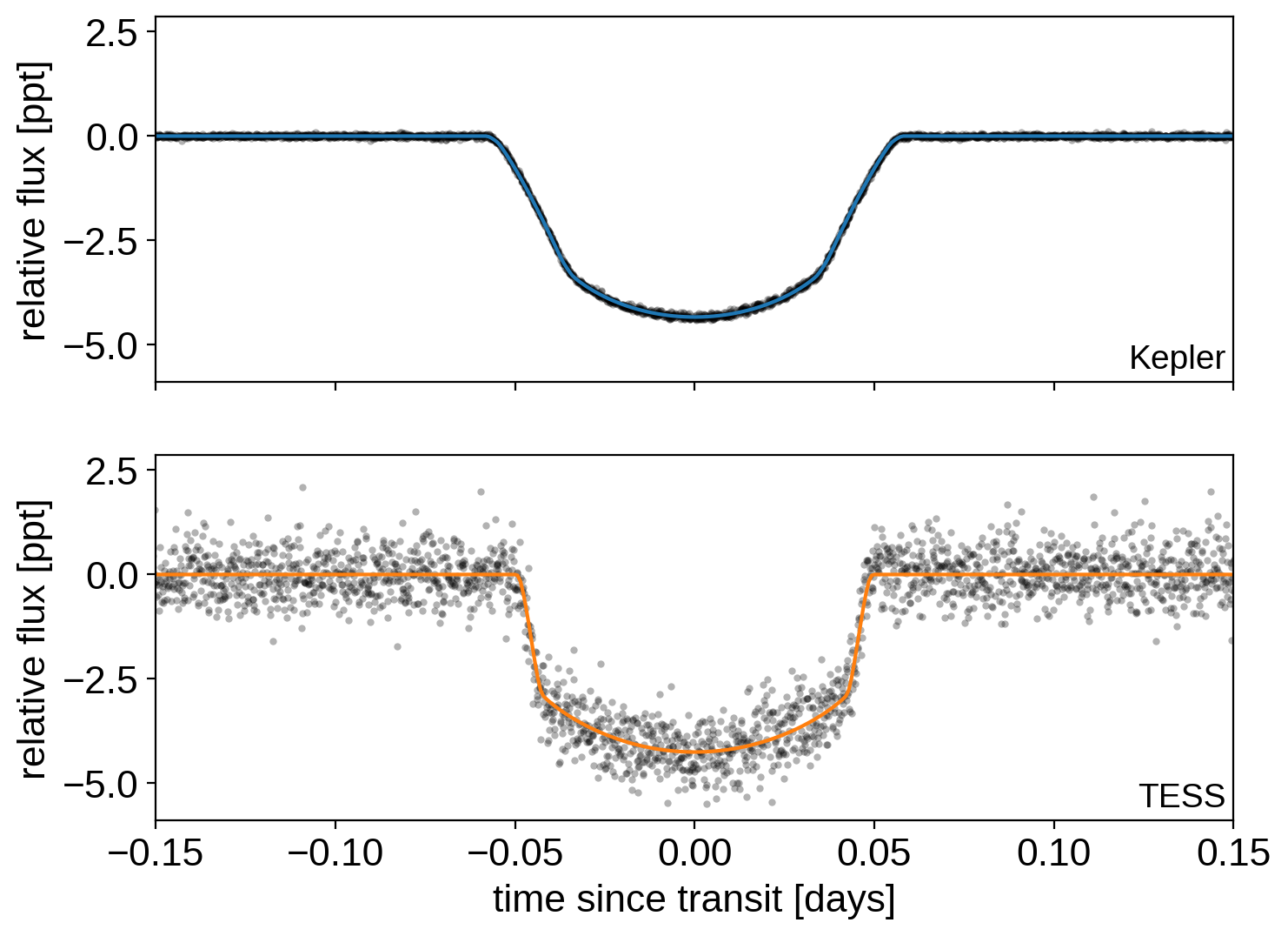
Here are the two phased light curves (with the Gaussian process model removed). We can see the effect of exposure time integration and the difference in photometric precision, but everything should be looking good!
dt = np.linspace(-0.2, 0.2, 500)

with model:
    trends = xo.eval_in_model([gp_preds[k] for k in datasets], map_soln)
    phase_curves = xo.eval_in_model([lc_models[k](t0 + dt) for k in datasets], map_soln)

fig, axes = plt.subplots(2, sharex=True, sharey=True, figsize=(8, 6))

for n, name in enumerate(datasets):
    ax = axes[n]

    x, y = datasets[name][:2]

    period = map_soln["period"]
    folded = (x - map_soln["t0"] + 0.5 * period) % period - 0.5 * period
    m = np.abs(folded) < 0.2
    ax.plot(
        folded[m],
        (y - trends[n] - map_soln[f"{name}_mean"])[m],
        ".k",
        alpha=0.3,
        mec="none",
    )
    ax.plot(dt, phase_curves[n] - map_soln[f"{name}_mean"], f"C{n}", label=name)
    ax.annotate(
        name,
        xy=(1, 0),
        xycoords="axes fraction",
        va="bottom",
        ha="right",
        xytext=(-3, 3),
        textcoords="offset points",
        fontsize=14,
    )

axes[-1].set_xlim(-0.15, 0.15)
axes[-1].set_xlabel("time since transit [days]")
for ax in axes:
    ax.set_ylabel("relative flux [ppt]")
Then we run the MCMC:
np.random.seed(11)
with model:
    trace = xo.sample(
        tune=3500, draws=3000, start=map_soln, chains=4, initial_accept=0.5
    )
Multiprocess sampling (4 chains in 4 jobs)
NUTS: [TESS_S_tot, TESS_sigma, TESS_approx_depth, TESS_u, TESS_mean, Kepler_S_tot, Kepler_sigma, Kepler_approx_depth, Kepler_u, Kepler_mean, ell, b, dur, t0, period]
Sampling 4 chains, 0 divergences: 100%|██████████| 26000/26000 [50:17<00:00,  8.62draws/s]
And check the convergence diagnostics:
pm.summary(trace)
| mean | sd | hpd_3% | hpd_97% | mcse_mean | mcse_sd | ess_mean | ess_sd | ess_bulk | ess_tail | r_hat | |
|---|---|---|---|---|---|---|---|---|---|---|---|
| t0 | 2011.505 | 0.000 | 2011.505 | 2011.505 | 0.000 | 0.000 | 18153.0 | 18153.0 | 18098.0 | 8866.0 | 1.0 |
| Kepler_mean | -0.331 | 0.206 | -0.706 | 0.070 | 0.001 | 0.001 | 22069.0 | 12535.0 | 22135.0 | 8035.0 | 1.0 |
| TESS_mean | 0.042 | 0.170 | -0.282 | 0.353 | 0.001 | 0.002 | 19215.0 | 5172.0 | 19307.0 | 8793.0 | 1.0 |
| period | 4.888 | 0.000 | 4.888 | 4.888 | 0.000 | 0.000 | 18665.0 | 18665.0 | 18655.0 | 9099.0 | 1.0 |
| dur | 0.092 | 0.000 | 0.092 | 0.092 | 0.000 | 0.000 | 4182.0 | 4180.0 | 4331.0 | 3982.0 | 1.0 |
| b | 0.407 | 0.038 | 0.337 | 0.481 | 0.001 | 0.000 | 3662.0 | 3662.0 | 4352.0 | 3136.0 | 1.0 |
| ell | 6.259 | 0.100 | 6.067 | 6.440 | 0.001 | 0.000 | 20423.0 | 20343.0 | 20502.0 | 9312.0 | 1.0 |
| Kepler_u[0] | 0.718 | 0.017 | 0.687 | 0.753 | 0.000 | 0.000 | 3997.0 | 3997.0 | 3987.0 | 3735.0 | 1.0 |
| Kepler_u[1] | -0.107 | 0.031 | -0.170 | -0.051 | 0.000 | 0.000 | 4193.0 | 4193.0 | 4245.0 | 4488.0 | 1.0 |
| Kepler_approx_depth | 0.003 | 0.000 | 0.003 | 0.003 | 0.000 | 0.000 | 12566.0 | 12566.0 | 12614.0 | 8206.0 | 1.0 |
| Kepler_ror | 0.060 | 0.000 | 0.059 | 0.061 | 0.000 | 0.000 | 3793.0 | 3793.0 | 4039.0 | 2824.0 | 1.0 |
| Kepler_sigma | 0.027 | 0.000 | 0.027 | 0.027 | 0.000 | 0.000 | 20268.0 | 20252.0 | 20292.0 | 8815.0 | 1.0 |
| Kepler_S_tot | 8.444 | 0.374 | 7.757 | 9.156 | 0.003 | 0.002 | 20105.0 | 19751.0 | 20355.0 | 8656.0 | 1.0 |
| TESS_u[0] | 0.731 | 0.074 | 0.592 | 0.862 | 0.001 | 0.001 | 5277.0 | 5162.0 | 5032.0 | 7130.0 | 1.0 |
| TESS_u[1] | -0.275 | 0.099 | -0.425 | -0.090 | 0.001 | 0.001 | 4588.0 | 4319.0 | 4063.0 | 4560.0 | 1.0 |
| TESS_approx_depth | 0.003 | 0.000 | 0.003 | 0.003 | 0.000 | 0.000 | 12159.0 | 12159.0 | 12158.0 | 8035.0 | 1.0 |
| TESS_ror | 0.060 | 0.000 | 0.060 | 0.061 | 0.000 | 0.000 | 5063.0 | 5063.0 | 5189.0 | 4361.0 | 1.0 |
| TESS_sigma | 0.232 | 0.004 | 0.225 | 0.239 | 0.000 | 0.000 | 21112.0 | 21112.0 | 21083.0 | 8529.0 | 1.0 |
| TESS_S_tot | 0.284 | 0.023 | 0.240 | 0.327 | 0.000 | 0.000 | 19602.0 | 18772.0 | 20198.0 | 8370.0 | 1.0 |
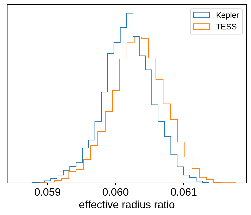
Since we fit for a radius ratio in each band, we can see if the transit depth is different in Kepler compared to TESS. The plot below demonstrates that there is no statistically significant difference between the radii measured in these two bands:
plt.hist(trace["Kepler_ror"], 30, density=True, histtype="step", label="Kepler")
plt.hist(trace["TESS_ror"], 30, density=True, histtype="step", label="TESS")
plt.yticks([])
plt.xlabel("effective radius ratio")
_ = plt.legend(fontsize=12)
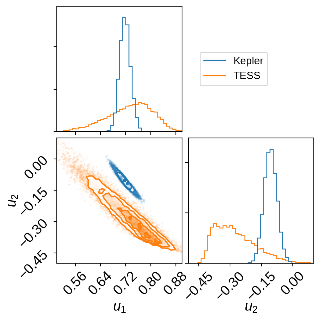
We can also compare the inferred limb-darkening coefficients:
import corner

fig = corner.corner(
    trace["TESS_u"], bins=40, color="C1", range=((0.5, 0.9), (-0.5, 0.1))
)
corner.corner(
    trace["Kepler_u"],
    bins=40,
    color="C0",
    fig=fig,
    labels=["$u_1$", "$u_2$"],
    range=((0.5, 0.9), (-0.5, 0.1)),
)
fig.axes[0].axvline(-1.0, color="C0", label="Kepler")
fig.axes[0].axvline(-1.0, color="C1", label="TESS")
_ = fig.axes[0].legend(fontsize=12, loc="center left", bbox_to_anchor=(1.1, 0.5))
As described in the Citing exoplanet & its dependencies tutorial, we can use
exoplanet.citations.get_citations_for_model() to construct an
acknowledgement and BibTeX listing that includes the relevant citations
for this model.
with model:
    txt, bib = xo.citations.get_citations_for_model()
print(txt)
This research made use of textsf{exoplanet} citep{exoplanet} and its
dependencies citep{exoplanet:astropy13, exoplanet:astropy18,
exoplanet:exoplanet, exoplanet:foremanmackey17, exoplanet:foremanmackey18,
exoplanet:pymc3, exoplanet:theano}.
print("\n".join(bib.splitlines()[:10]) + "\n...")
@misc{exoplanet:exoplanet,
  author = {Daniel Foreman-Mackey and Rodrigo Luger and Ian Czekala and
            Eric Agol and Adrian Price-Whelan and Tom Barclay},
   title = {exoplanet-dev/exoplanet v0.3.2},
   month = may,
    year = 2020,
     doi = {10.5281/zenodo.1998447},
     url = {https://doi.org/10.5281/zenodo.1998447}
}
...