Note
This tutorial was generated from an IPython notebook that can be downloaded here.
In this case study, we will look at how we can use exoplanet and PyMC3 to combine datasets from different RV instruments to fit the orbit of an exoplanet system. Before getting started, I want to emphasize that the exoplanet code doesn’t have strong opinions about how your data are collected, it only provides extensions that allow PyMC3 to evaluate some astronomy-specific functions. This means that you can build any kind of observation model that PyMC3 supports, and support for multiple instruments isn’t really a feature of exoplanet, even though it is easy to implement.
For the example, we’ll use public observations of Pi Mensae which hosts two planets, but we’ll ignore the inner planet because the significance of the RV signal is small enough that it won’t affect our results. The datasets that we’ll use are from the Anglo-Australian Planet Search (AAT) and the HARPS archive. As is commonly done, we will treat the HARPS observations as two independent datasets split in June 2015 when the HARPS hardware was upgraded. Therefore, we’ll consider three datasets that we will allow to have different instrumental parameters (RV offset and jitter), but shared orbital parameters and stellar variability. In some cases you might also want to have a different astrophyscial variability model for each instrument (if, for example, the observations are made in very different bands), but we’ll keep things simple for this example.
The AAT data are available from The Exoplanet Archive and the HARPS observations can be downloaded from the ESO Archive. For the sake of simplicity, we have extracted the HARPS RVs from the archive in advance using Megan Bedell’s harps_tools library.
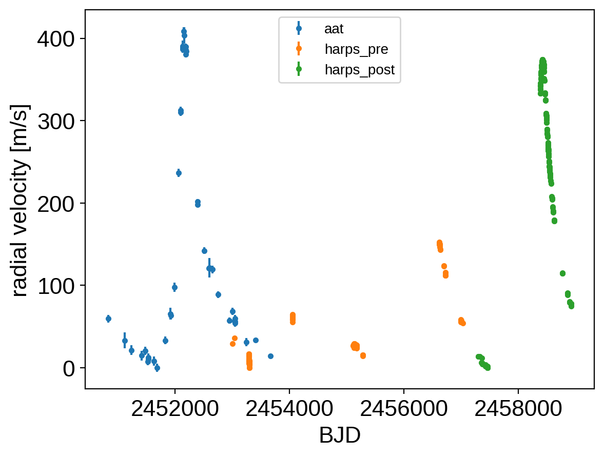
To start, download the data and plot them with a (very!) rough zero point correction.
import numpy as np
import pandas as pd
from astropy.io import ascii

aat = ascii.read(
    "https://exoplanetarchive.ipac.caltech.edu/data/ExoData/0026/0026394/data/UID_0026394_RVC_001.tbl"
)
harps = pd.read_csv(
    "https://raw.githubusercontent.com/exoplanet-dev/case-studies/master/data/pi_men_harps_rvs.csv",
    skiprows=1,
)
harps = harps.rename(lambda x: x.strip().strip("#"), axis=1)
harps_post = np.array(harps.date > "2015-07-01", dtype=int)

t = np.concatenate((aat["JD"], harps["bjd"]))
rv = np.concatenate((aat["Radial_Velocity"], harps["rv"]))
rv_err = np.concatenate((aat["Radial_Velocity_Uncertainty"], harps["e_rv"]))
inst_id = np.concatenate((np.zeros(len(aat), dtype=int), harps_post + 1))

inds = np.argsort(t)
t = np.ascontiguousarray(t[inds], dtype=float)
rv = np.ascontiguousarray(rv[inds], dtype=float)
rv_err = np.ascontiguousarray(rv_err[inds], dtype=float)
inst_id = np.ascontiguousarray(inst_id[inds], dtype=int)

inst_names = ["aat", "harps_pre", "harps_post"]
num_inst = len(inst_names)

for i, name in enumerate(inst_names):
    m = inst_id == i
    plt.errorbar(t[m], rv[m] - np.min(rv[m]), yerr=rv_err[m], fmt=".", label=name)

plt.legend(fontsize=10)
plt.xlabel("BJD")
_ = plt.ylabel("radial velocity [m/s]")
Then set up the probabilistic model. Most of this is similar to the model in the Radial velocity fitting tutorial, but there are a few changes to highlight:
import pymc3 as pm
import exoplanet as xo
import theano.tensor as tt

with pm.Model() as model:

    # Parameters describing the orbit
    K = pm.Lognormal("K", mu=np.log(300), sigma=10)
    P = pm.Lognormal("P", mu=np.log(2093.07), sigma=10)

    ecs = xo.UnitDisk("ecs", testval=np.array([0.7, -0.3]))
    ecc = pm.Deterministic("ecc", tt.sum(ecs ** 2))
    omega = pm.Deterministic("omega", tt.arctan2(ecs[1], ecs[0]))
    phase = xo.UnitUniform("phase")
    tp = pm.Deterministic("tp", 0.5 * (t.min() + t.max()) + phase * P)

    orbit = xo.orbits.KeplerianOrbit(period=P, t_periastron=tp, ecc=ecc, omega=omega)

    # Noise model parameters
    S_tot = pm.Lognormal("S_tot", mu=np.log(10), sigma=50)
    ell = pm.Lognormal("ell", mu=np.log(50), sigma=50)

    # Per instrument parameters
    means = pm.Normal(
        "means",
        mu=np.array([np.median(rv[inst_id == i]) for i in range(num_inst)]),
        sigma=200,
        shape=num_inst,
    )
    sigmas = pm.HalfNormal("sigmas", sigma=10, shape=num_inst)

    # Compute the RV offset and jitter for each data point depending on its instrument
    mean = tt.zeros(len(t))
    diag = tt.zeros(len(t))
    for i in range(len(inst_names)):
        mean += means[i] * (inst_id == i)
        diag += (rv_err ** 2 + sigmas[i] ** 2) * (inst_id == i)
    pm.Deterministic("mean", mean)
    pm.Deterministic("diag", diag)

    def rv_model(x):
        return orbit.get_radial_velocity(x, K=K)

    kernel = xo.gp.terms.SHOTerm(S_tot=S_tot, w0=2 * np.pi / ell, Q=1.0 / 3)
    gp = xo.gp.GP(kernel, t, diag, mean=rv_model)
    gp.marginal("obs", observed=rv - mean)
    pm.Deterministic("gp_pred", gp.predict())

    map_soln = model.test_point
    map_soln = xo.optimize(map_soln, [means])
    map_soln = xo.optimize(map_soln, [means, phase])
    map_soln = xo.optimize(map_soln, [means, phase, K])
    map_soln = xo.optimize(map_soln, [means, tp, K, P, ecs])
    map_soln = xo.optimize(map_soln, [sigmas, S_tot, ell])
    map_soln = xo.optimize(map_soln)
optimizing logp for variables: [means]
14it [00:08,  1.59it/s, logp=-1.137136e+04]
message: Optimization terminated successfully.
logp: -18094.31463741889 -> -11371.356631997516
optimizing logp for variables: [phase, means]
134it [00:00, 173.21it/s, logp=-1.123946e+04]
message: Desired error not necessarily achieved due to precision loss.
logp: -11371.356631997516 -> -11239.464875071475
optimizing logp for variables: [K, phase, means]
27it [00:00, 38.58it/s, logp=-1.509021e+03]
message: Optimization terminated successfully.
logp: -11239.464875071475 -> -1509.0207936381803
optimizing logp for variables: [ecs, P, K, phase, means]
93it [00:00, 133.99it/s, logp=-1.329611e+03]
message: Optimization terminated successfully.
logp: -1509.0207936381803 -> -1329.6106228736105
optimizing logp for variables: [ell, S_tot, sigmas]
22it [00:00, 41.15it/s, logp=-8.455534e+02]
message: Optimization terminated successfully.
logp: -1329.6106228736105 -> -845.553449086343
optimizing logp for variables: [sigmas, means, ell, S_tot, phase, ecs, P, K]
101it [00:00, 114.02it/s, logp=-8.428013e+02]
message: Desired error not necessarily achieved due to precision loss.
logp: -845.553449086343 -> -842.8013426538246
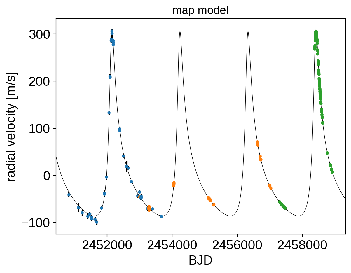
After fitting for the parameters that maximize the posterior probability, we can plot this model to make sure that things are looking reasonable:
t_pred = np.linspace(t.min() - 400, t.max() + 400, 5000)
with model:
    plt.plot(t_pred, xo.eval_in_model(rv_model(t_pred), map_soln), "k", lw=0.5)

detrended = rv - map_soln["mean"] - map_soln["gp_pred"]
plt.errorbar(t, detrended, yerr=rv_err, fmt=",k")
plt.scatter(t, detrended, c=inst_id, s=8, zorder=100, cmap="tab10", vmin=0, vmax=10)
plt.xlim(t_pred.min(), t_pred.max())
plt.xlabel("BJD")
plt.ylabel("radial velocity [m/s]")
_ = plt.title("map model", fontsize=14)
That looks fine, so now we can run the MCMC sampler:
np.random.seed(39091)
with model:
    trace = xo.sample(tune=3500, draws=3000, start=map_soln, chains=4)
Multiprocess sampling (4 chains in 4 jobs)
NUTS: [sigmas, means, ell, S_tot, phase, ecs, P, K]
Sampling 4 chains, 0 divergences: 100%|██████████| 26000/26000 [01:17<00:00, 337.27draws/s]
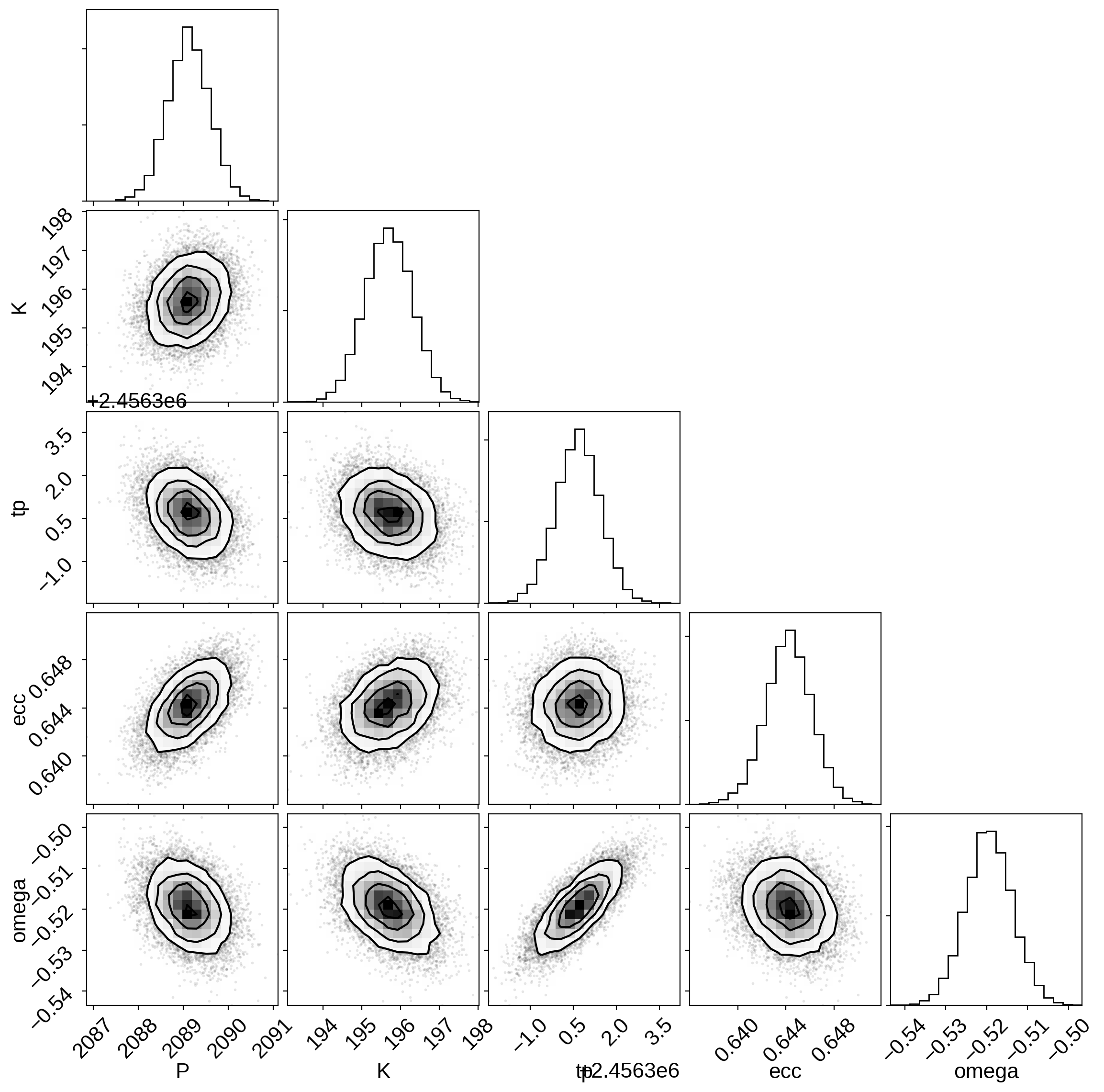
Then we can look at some summaries of the trace and the constraints on some of the key parameters:
import corner

corner.corner(pm.trace_to_dataframe(trace, varnames=["P", "K", "tp", "ecc", "omega"]))

pm.summary(trace, var_names=["P", "K", "tp", "ecc", "omega", "means", "sigmas"])
| mean | sd | hpd_3% | hpd_97% | mcse_mean | mcse_sd | ess_mean | ess_sd | ess_bulk | ess_tail | r_hat | |
|---|---|---|---|---|---|---|---|---|---|---|---|
| P | 2089.116 | 0.469 | 2088.250 | 2090.009 | 0.004 | 0.002 | 17573.0 | 17573.0 | 17624.0 | 8756.0 | 1.0 |
| K | 195.693 | 0.620 | 194.526 | 196.843 | 0.005 | 0.003 | 16656.0 | 16650.0 | 16665.0 | 8997.0 | 1.0 |
| tp | 2456300.672 | 0.784 | 2456299.179 | 2456302.128 | 0.006 | 0.004 | 16779.0 | 16779.0 | 16788.0 | 8497.0 | 1.0 |
| ecc | 0.644 | 0.002 | 0.640 | 0.648 | 0.000 | 0.000 | 16895.0 | 16895.0 | 16975.0 | 8431.0 | 1.0 |
| omega | -0.519 | 0.006 | -0.530 | -0.508 | 0.000 | 0.000 | 17202.0 | 17202.0 | 17181.0 | 8596.0 | 1.0 |
| means[0] | 1.779 | 1.038 | -0.190 | 3.728 | 0.008 | 0.006 | 17485.0 | 13359.0 | 17499.0 | 8418.0 | 1.0 |
| means[1] | 10709.375 | 0.531 | 10708.323 | 10710.325 | 0.004 | 0.003 | 17390.0 | 17390.0 | 17425.0 | 8005.0 | 1.0 |
| means[2] | 10729.159 | 0.681 | 10727.890 | 10730.457 | 0.005 | 0.004 | 18289.0 | 18289.0 | 18274.0 | 9179.0 | 1.0 |
| sigmas[0] | 3.022 | 1.420 | 0.032 | 5.219 | 0.018 | 0.013 | 6323.0 | 6323.0 | 5844.0 | 3482.0 | 1.0 |
| sigmas[1] | 0.877 | 0.109 | 0.684 | 1.093 | 0.001 | 0.001 | 17362.0 | 16324.0 | 17823.0 | 8740.0 | 1.0 |
| sigmas[2] | 0.508 | 0.045 | 0.429 | 0.594 | 0.000 | 0.000 | 17359.0 | 17190.0 | 17258.0 | 8767.0 | 1.0 |
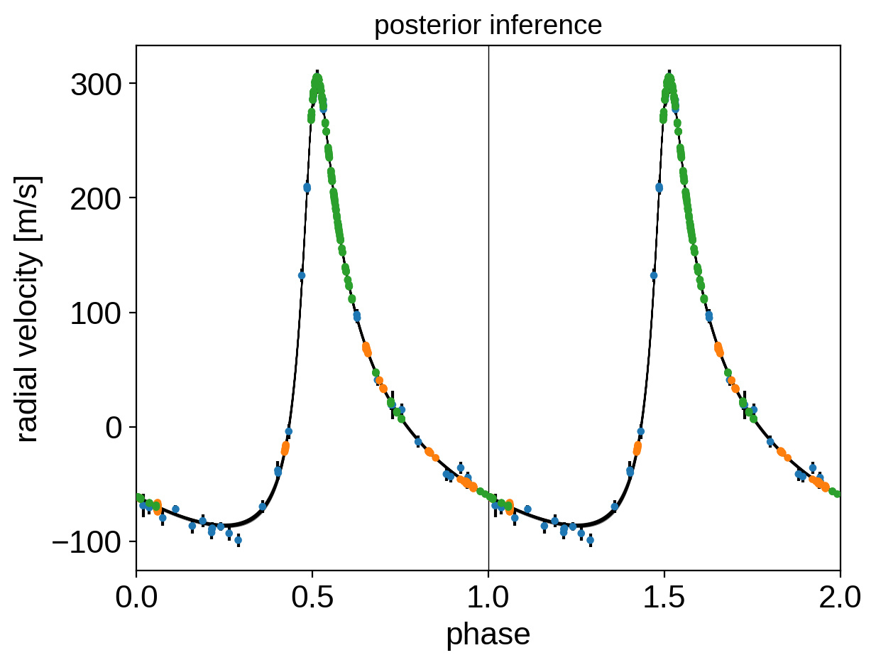
And finally we can plot the phased RV curve and overplot our posterior inference:
mu = np.mean(trace["mean"] + trace["gp_pred"], axis=0)
mu_var = np.var(trace["mean"], axis=0)
jitter_var = np.median(trace["diag"], axis=0)
period = np.median(trace["P"])
tp = np.median(trace["tp"])

detrended = rv - mu
folded = ((t - tp + 0.5 * period) % period) / period
plt.errorbar(folded, detrended, yerr=np.sqrt(mu_var + jitter_var), fmt=",k")
plt.scatter(
    folded, detrended, c=inst_id, s=8, zorder=100, cmap="tab10", vmin=0, vmax=10
)
plt.errorbar(folded + 1, detrended, yerr=np.sqrt(mu_var + jitter_var), fmt=",k")
plt.scatter(
    folded + 1, detrended, c=inst_id, s=8, zorder=100, cmap="tab10", vmin=0, vmax=10
)

t_phase = np.linspace(-0.5, 0.5, 5000)
with model:
    func = xo.get_theano_function_for_var(rv_model(model.P * t_phase + model.tp))
    for point in xo.get_samples_from_trace(trace, 100):
        args = xo.get_args_for_theano_function(point)
        x, y = t_phase + 0.5, func(*args)
        plt.plot(x, y, "k", lw=0.5, alpha=0.5)
        plt.plot(x + 1, y, "k", lw=0.5, alpha=0.5)
plt.axvline(1, color="k", lw=0.5)
plt.xlim(0, 2)
plt.xlabel("phase")
plt.ylabel("radial velocity [m/s]")
_ = plt.title("posterior inference", fontsize=14)
As described in the Citing exoplanet & its dependencies tutorial, we can use
exoplanet.citations.get_citations_for_model() to construct an
acknowledgement and BibTeX listing that includes the relevant citations
for this model.
with model:
    txt, bib = xo.citations.get_citations_for_model()
print(txt)
This research made use of textsf{exoplanet} citep{exoplanet} and its
dependencies citep{exoplanet:astropy13, exoplanet:astropy18,
exoplanet:exoplanet, exoplanet:foremanmackey17, exoplanet:foremanmackey18,
exoplanet:pymc3, exoplanet:theano}.
print("\n".join(bib.splitlines()[:10]) + "\n...")
@misc{exoplanet:exoplanet,
  author = {Daniel Foreman-Mackey and Rodrigo Luger and Ian Czekala and
            Eric Agol and Adrian Price-Whelan and Tom Barclay},
   title = {exoplanet-dev/exoplanet v0.3.2},
   month = may,
    year = 2020,
     doi = {10.5281/zenodo.1998447},
     url = {https://doi.org/10.5281/zenodo.1998447}
}
...