Note
This tutorial was generated from an IPython notebook that can be downloaded here.
Note
You will need exoplanet version 0.2.6 or later to run this tutorial.
In this tutorial, we will fit the TESS light curve for a known transiting planet. While the Fitting TESS data tutorial goes through the full details of an end-to-end fit, this tutorial is significantly faster to run and it can give pretty excellent results depending on your goals. Some of the main differences are:
We’ll fit the planet in the HD 118203 (TIC 286923464) system that was found to transit by Pepper et al. (2019) because it is on an eccentric orbit so assumption #2 above is not valid.
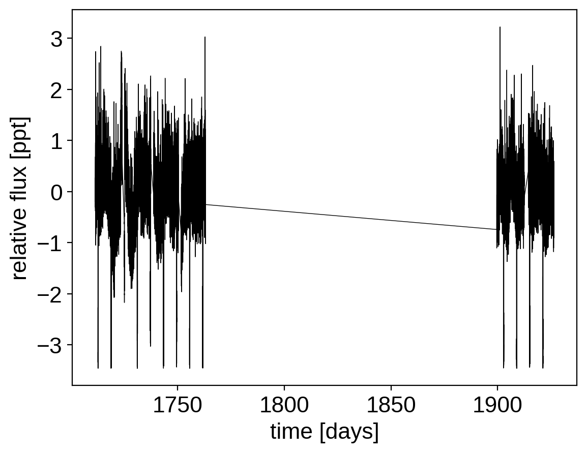
First, let’s download the TESS light curve using lightkurve:
import numpy as np
import lightkurve as lk
import matplotlib.pyplot as plt

lcfs = lk.search_lightcurvefile("TIC 286923464", mission="TESS").download_all()
lc = lcfs.PDCSAP_FLUX.stitch()
lc = lc.remove_nans().remove_outliers()

x = np.ascontiguousarray(lc.time, dtype=np.float64)
y = np.ascontiguousarray(1e3 * (lc.flux - 1), dtype=np.float64)
yerr = np.ascontiguousarray(1e3 * lc.flux_err, dtype=np.float64)

texp = np.min(np.diff(x))

plt.plot(x, y, "k", linewidth=0.5)
plt.xlabel("time [days]")
plt.ylabel("relative flux [ppt]");
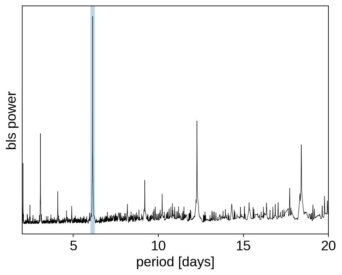
Then, find the period, phase and depth of the transit using box least squares:
import exoplanet as xo

pg = xo.estimators.bls_estimator(x, y, yerr, min_period=2, max_period=20)

peak = pg["peak_info"]
period_guess = peak["period"]
t0_guess = peak["transit_time"]
depth_guess = peak["depth"]

plt.plot(pg["bls"].period, pg["bls"].power, "k", linewidth=0.5)
plt.axvline(period_guess, alpha=0.3, linewidth=5)
plt.xlabel("period [days]")
plt.ylabel("bls power")
plt.yticks([])
plt.xlim(pg["bls"].period.min(), pg["bls"].period.max());
Then, for efficiency purposes, let’s extract just the data within 0.25 days of the transits:
transit_mask = (
    np.abs((x - t0_guess + 0.5 * period_guess) % period_guess - 0.5 * period_guess)
    < 0.25
)
x = np.ascontiguousarray(x[transit_mask])
y = np.ascontiguousarray(y[transit_mask])
yerr = np.ascontiguousarray(yerr[transit_mask])

plt.figure(figsize=(8, 4))
x_fold = (x - t0_guess + 0.5 * period_guess) % period_guess - 0.5 * period_guess
plt.scatter(x_fold, y, c=x, s=3)
plt.xlabel("time since transit [days]")
plt.ylabel("relative flux [ppt]")
plt.colorbar(label="time [days]")
plt.xlim(-0.25, 0.25);
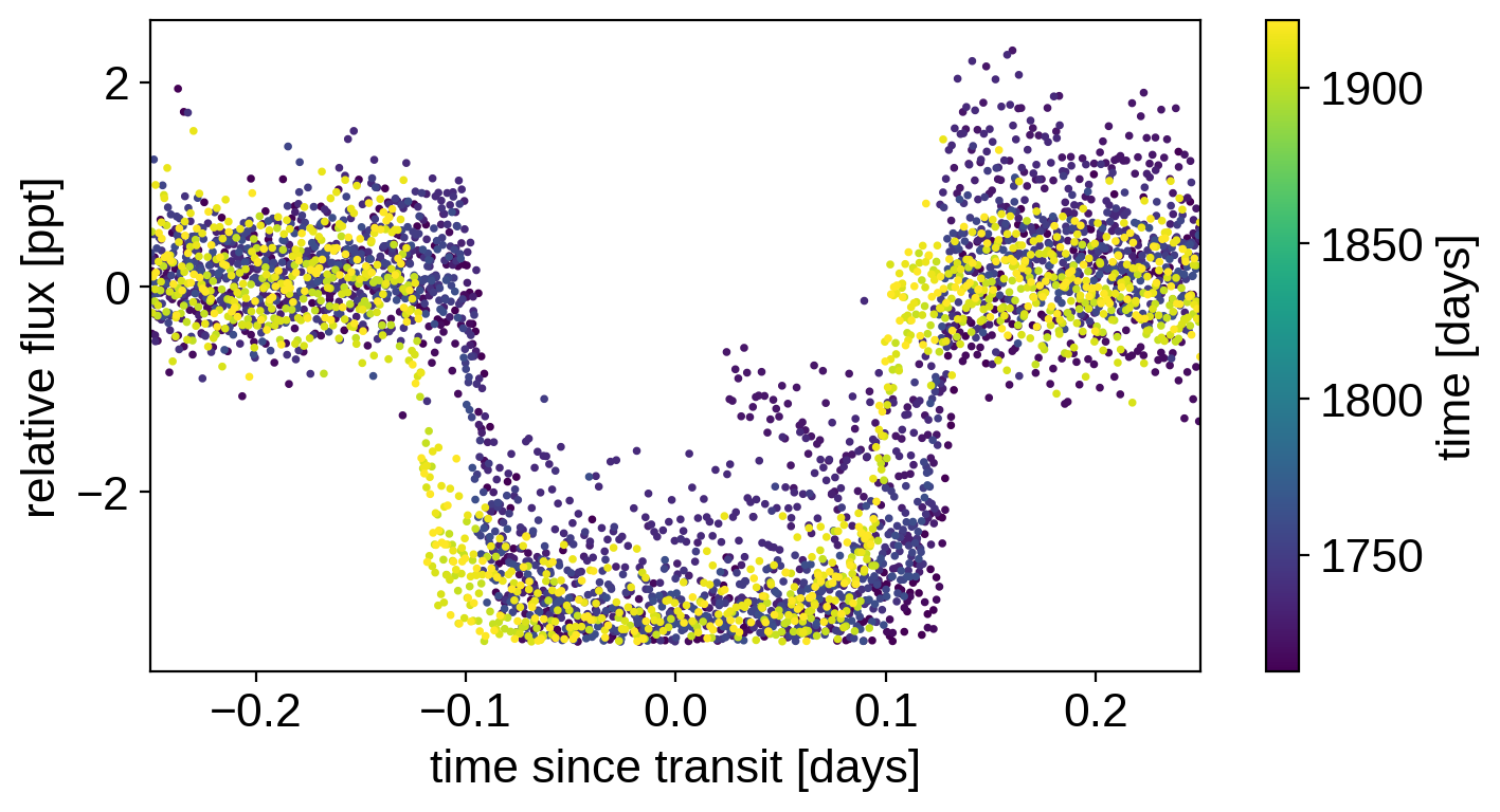
That looks a little janky, but it’s good enough for now.
Here’s how we set up the PyMC3 model in this case:
import pymc3 as pm
import theano.tensor as tt

with pm.Model() as model:

    # Stellar parameters
    mean = pm.Normal("mean", mu=0.0, sigma=10.0)
    u = xo.distributions.QuadLimbDark("u")
    star_params = [mean, u]

    # Gaussian process noise model
    sigma = pm.InverseGamma("sigma", alpha=3.0, beta=2 * np.median(yerr))
    log_Sw4 = pm.Normal("log_Sw4", mu=0.0, sigma=10.0)
    log_w0 = pm.Normal("log_w0", mu=np.log(2 * np.pi / 10.0), sigma=10.0)
    kernel = xo.gp.terms.SHOTerm(log_Sw4=log_Sw4, log_w0=log_w0, Q=1.0 / 3)
    noise_params = [sigma, log_Sw4, log_w0]

    # Planet parameters
    log_ror = pm.Normal("log_ror", mu=0.5 * np.log(depth_guess * 1e-3), sigma=10.0)
    ror = pm.Deterministic("ror", tt.exp(log_ror))

    # Orbital parameters
    log_period = pm.Normal("log_period", mu=np.log(period_guess), sigma=1.0)
    t0 = pm.Normal("t0", mu=t0_guess, sigma=1.0)
    log_dur = pm.Normal("log_dur", mu=np.log(0.1), sigma=10.0)
    b = xo.distributions.ImpactParameter("b", ror=ror)

    period = pm.Deterministic("period", tt.exp(log_period))
    dur = pm.Deterministic("dur", tt.exp(log_dur))

    # Set up the orbit
    orbit = xo.orbits.KeplerianOrbit(period=period, duration=dur, t0=t0, b=b)

    # We're going to track the implied density for reasons that will become clear later
    pm.Deterministic("rho_circ", orbit.rho_star)

    # Set up the mean transit model
    star = xo.LimbDarkLightCurve(u)

    def lc_model(t):
        return mean + 1e3 * tt.sum(
            star.get_light_curve(orbit=orbit, r=ror, t=t), axis=-1
        )

    # Finally the GP observation model
    gp = xo.gp.GP(kernel, x, yerr ** 2 + sigma ** 2, mean=lc_model)
    gp.marginal("obs", observed=y)

    # Double check that everything looks good - we shouldn't see any NaNs!
    print(model.check_test_point())

    # Optimize the model
    map_soln = model.test_point
    map_soln = xo.optimize(map_soln, [sigma])
    map_soln = xo.optimize(map_soln, [log_ror, b, log_dur])
    map_soln = xo.optimize(map_soln, noise_params)
    map_soln = xo.optimize(map_soln, star_params)
    map_soln = xo.optimize(map_soln)
mean                   -3.22
u_quadlimbdark__       -2.77
sigma_log__            -0.53
log_Sw4                -3.22
log_w0                 -3.22
log_ror                -3.22
log_period             -0.92
t0                     -0.92
log_dur                -3.22
b_impact__             -1.39
obs                -24037.81
Name: Log-probability of test_point, dtype: float64
optimizing logp for variables: [sigma]
16it [00:01,  9.51it/s, logp=-6.491897e+03]
message: Optimization terminated successfully.
logp: -24060.450789871506 -> -6491.896832790021
optimizing logp for variables: [log_dur, b, log_ror]
21it [00:00, 105.31it/s, logp=-4.926412e+03]
message: Optimization terminated successfully.
logp: -6491.896832790021 -> -4926.412276779751
optimizing logp for variables: [log_w0, log_Sw4, sigma]
79it [00:00, 145.63it/s, logp=-1.872912e+03]
message: Optimization terminated successfully.
logp: -4926.412276779751 -> -1872.9123033179976
optimizing logp for variables: [u, mean]
13it [00:00, 76.15it/s, logp=-1.867587e+03]
message: Optimization terminated successfully.
logp: -1872.9123033179976 -> -1867.58739329712
optimizing logp for variables: [b, log_dur, t0, log_period, log_ror, log_w0, log_Sw4, sigma, u, mean]
134it [00:00, 236.16it/s, logp=-1.381469e+03]
message: Desired error not necessarily achieved due to precision loss.
logp: -1867.58739329712 -> -1381.4688211234925
Now we can plot our initial model:
with model:
    gp_pred, lc_pred = xo.eval_in_model([gp.predict(), lc_model(x)], map_soln)

plt.figure(figsize=(8, 4))
x_fold = (x - map_soln["t0"] + 0.5 * map_soln["period"]) % map_soln[
    "period"
] - 0.5 * map_soln["period"]
inds = np.argsort(x_fold)
plt.scatter(x_fold, y - gp_pred - map_soln["mean"], c=x, s=3)
plt.plot(x_fold[inds], lc_pred[inds] - map_soln["mean"], "k")
plt.xlabel("time since transit [days]")
plt.ylabel("relative flux [ppt]")
plt.colorbar(label="time [days]")
plt.xlim(-0.25, 0.25);
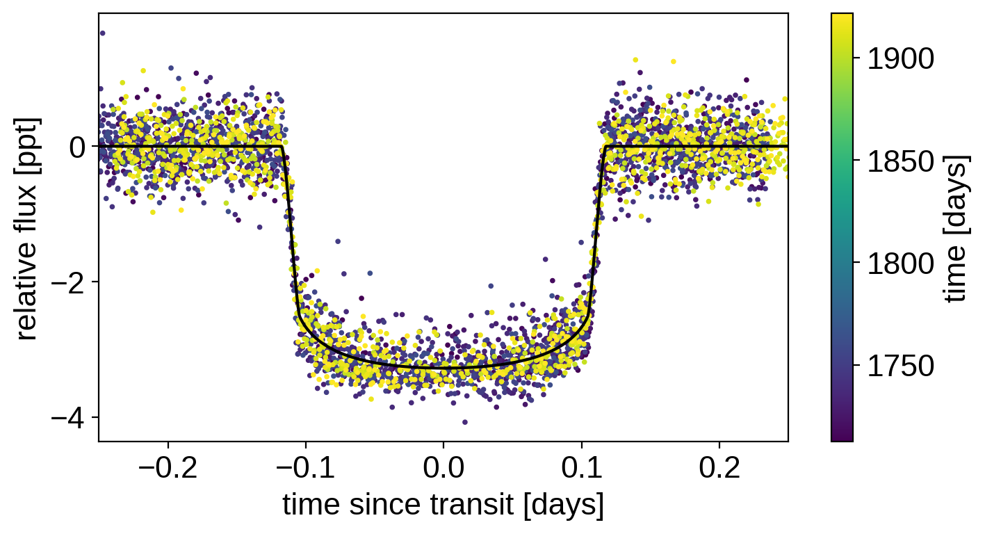
That looks better!
Now on to sampling:
np.random.seed(286923464)
with model:
    trace = xo.sample(tune=2000, draws=2000, start=map_soln, chains=4)
Multiprocess sampling (4 chains in 4 jobs)
NUTS: [b, log_dur, t0, log_period, log_ror, log_w0, log_Sw4, sigma, u, mean]
Sampling 4 chains, 0 divergences: 100%|██████████| 16000/16000 [03:07<00:00, 85.25draws/s]
Then we can take a look at the summary statistics:
pm.summary(trace)
| mean | sd | hpd_3% | hpd_97% | mcse_mean | mcse_sd | ess_mean | ess_sd | ess_bulk | ess_tail | r_hat | |
|---|---|---|---|---|---|---|---|---|---|---|---|
| mean | 0.217 | 0.103 | 0.015 | 0.401 | 0.001 | 0.001 | 6905.0 | 6435.0 | 7005.0 | 5079.0 | 1.0 |
| log_Sw4 | 6.131 | 0.339 | 5.503 | 6.776 | 0.004 | 0.003 | 8900.0 | 8807.0 | 8908.0 | 5655.0 | 1.0 |
| log_w0 | 2.187 | 0.172 | 1.861 | 2.498 | 0.002 | 0.001 | 8009.0 | 8009.0 | 8041.0 | 5592.0 | 1.0 |
| log_ror | -2.913 | 0.007 | -2.926 | -2.898 | 0.000 | 0.000 | 6984.0 | 6984.0 | 7017.0 | 5499.0 | 1.0 |
| log_period | 1.814 | 0.000 | 1.814 | 1.814 | 0.000 | 0.000 | 9271.0 | 9271.0 | 9276.0 | 6378.0 | 1.0 |
| t0 | 1712.662 | 0.000 | 1712.662 | 1712.662 | 0.000 | 0.000 | 9552.0 | 9552.0 | 9546.0 | 6070.0 | 1.0 |
| log_dur | -1.504 | 0.002 | -1.507 | -1.500 | 0.000 | 0.000 | 8222.0 | 8221.0 | 8224.0 | 5774.0 | 1.0 |
| u[0] | 0.173 | 0.076 | 0.029 | 0.309 | 0.001 | 0.001 | 5429.0 | 5429.0 | 4913.0 | 2354.0 | 1.0 |
| u[1] | 0.252 | 0.104 | 0.063 | 0.447 | 0.001 | 0.001 | 5715.0 | 4661.0 | 5521.0 | 3815.0 | 1.0 |
| sigma | 0.159 | 0.008 | 0.145 | 0.173 | 0.000 | 0.000 | 8942.0 | 8942.0 | 8949.0 | 5887.0 | 1.0 |
| ror | 0.054 | 0.000 | 0.054 | 0.055 | 0.000 | 0.000 | 6979.0 | 6975.0 | 7017.0 | 5499.0 | 1.0 |
| b | 0.214 | 0.094 | 0.020 | 0.357 | 0.002 | 0.001 | 2096.0 | 2096.0 | 2356.0 | 1938.0 | 1.0 |
| period | 6.135 | 0.000 | 6.135 | 6.135 | 0.000 | 0.000 | 9271.0 | 9271.0 | 9276.0 | 6378.0 | 1.0 |
| dur | 0.222 | 0.000 | 0.221 | 0.223 | 0.000 | 0.000 | 8224.0 | 8224.0 | 8224.0 | 5774.0 | 1.0 |
| rho_circ | 0.316 | 0.018 | 0.285 | 0.345 | 0.000 | 0.000 | 3136.0 | 2964.0 | 2539.0 | 2750.0 | 1.0 |
And plot the posterior covariances compared to the values from Pepper et al. (2019):
import corner
import astropy.units as u

samples = pm.trace_to_dataframe(trace, varnames=["period", "ror", "b"])
corner.corner(samples, truths=[6.134980, 0.05538, 0.125]);
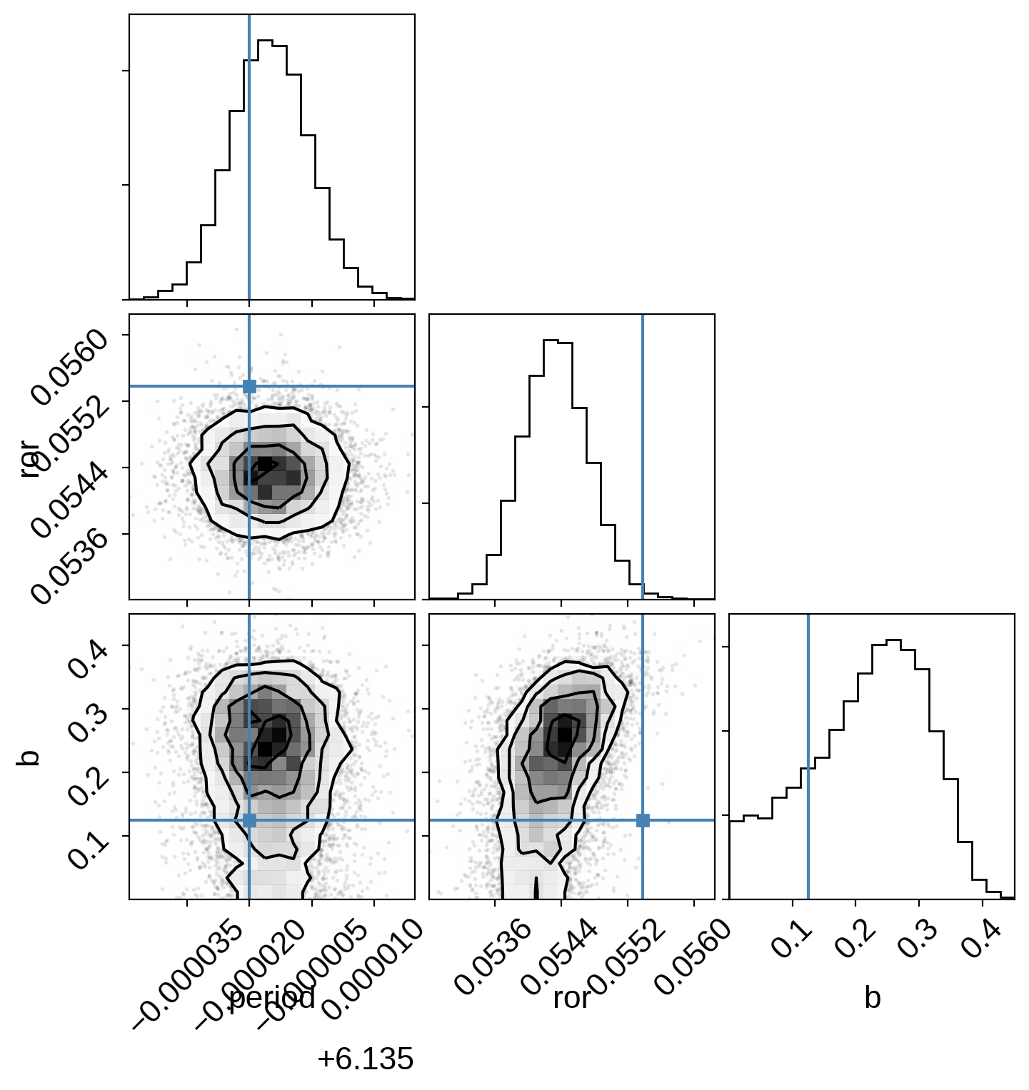
As discussed above, we fit this model assuming a circular orbit which speeds things up for a few reasons. First, setting eccentricity to zero means that the orbital dynamics are much simpler and more computationally efficient, since we don’t need to solve Kepler’s equation numerically. But this isn’t actually the main effect! Instead the bigger issues come from the fact that the degeneracies between eccentricity, arrgument of periasteron, impact parameter, and planet radius are hard for the sampler to handle, causing the sampler’s performance to plummet. In this case, by fitting with a circular orbit where duration is one of the parameters, everything is well behaved and the sampler runs faster.
But, in this case, the planet is actually on an eccentric orbit, so that assumption isn’t justified. It has been recognized by various researchers over the years (I first learned about this from Bekki Dawson) that, to first order, the eccentricity mainly just changes the transit duration. The key realization is that this can be thought of as a change in the impled density of the star. Therefore, if you fit the transit using stellar density (or duration, in this case) as one of the parameters (note: you must have a different stellar density parameter for each planet if there are more than one), you can use an independent measurement of the stellar density to infer the eccentricity of the orbit after the fact. All the details are described in Dawson & Johnson (2012), but here’s how you can do this here using the stellar density listed in the TESS input catalog:
from astroquery.mast import Catalogs

star = Catalogs.query_object("TIC 286923464", catalog="TIC", radius=0.001)
tic_rho_star = float(star["rho"]), float(star["e_rho"])
print("rho_star = {0} ± {1}".format(*tic_rho_star))

# Extract the implied density from the fit
rho_circ = np.repeat(trace["rho_circ"], 100)

# Sample eccentricity and omega from their priors (the math might
# be a little more subtle for more informative priors, but I leave
# that as an exercise for the reader...)
ecc = np.random.uniform(0, 1, len(rho_circ))
omega = np.random.uniform(-np.pi, np.pi, len(rho_circ))

# Compute the "g" parameter from Dawson & Johnson and what true
# density that implies
g = (1 + ecc * np.sin(omega)) / np.sqrt(1 - ecc ** 2)
rho = rho_circ / g ** 3

# Re-weight these samples to get weighted posterior samples
log_weights = -0.5 * ((rho - tic_rho_star[0]) / tic_rho_star[1]) ** 2
weights = np.exp(log_weights - np.max(log_weights))

# Estimate the expected posterior quantiles
q = corner.quantile(ecc, [0.16, 0.5, 0.84], weights=weights)
print("eccentricity = {0:.2f} +{1[1]:.2f} -{1[0]:.2f}".format(q[1], np.diff(q)))

corner.corner(
    np.vstack((ecc, omega)).T,
    weights=weights,
    truths=[0.316, None],
    plot_datapoints=False,
    labels=["eccentricity", "omega"],
);
rho_star = 0.121689 ± 0.0281776
eccentricity = 0.45 +0.25 -0.14
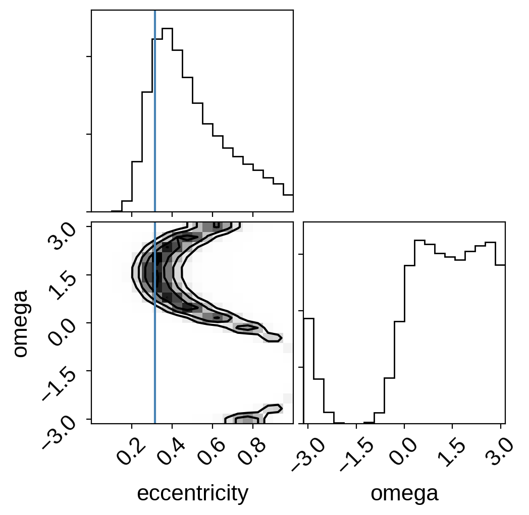
As you can see, this eccentricity estimate is consistent (albeit with large uncertainties) with the value that Pepper et al. (2019) measure using radial velocities and it is definitely clear that this planet is not on a circular orbit.
As described in the Citing exoplanet & its dependencies tutorial, we can use
exoplanet.citations.get_citations_for_model() to construct an
acknowledgement and BibTeX listing that includes the relevant citations
for this model.
with model:
    txt, bib = xo.citations.get_citations_for_model()
print(txt)
This research made use of textsf{exoplanet} citep{exoplanet} and its
dependencies citep{exoplanet:agol19, exoplanet:astropy13, exoplanet:astropy18,
exoplanet:exoplanet, exoplanet:foremanmackey17, exoplanet:foremanmackey18,
exoplanet:kipping13, exoplanet:luger18, exoplanet:pymc3, exoplanet:theano}.
print("\n".join(bib.splitlines()[:10]) + "\n...")
@misc{exoplanet:exoplanet,
  author = {Daniel Foreman-Mackey and Rodrigo Luger and Ian Czekala and
            Eric Agol and Adrian Price-Whelan and Tom Barclay},
   title = {exoplanet-dev/exoplanet v0.3.2},
   month = may,
    year = 2020,
     doi = {10.5281/zenodo.1998447},
     url = {https://doi.org/10.5281/zenodo.1998447}
}
...